
-
摘要:
为应对光照条件复杂多变下的多场景视觉感知挑战,本文提出了一种照度条件自适应的粒度渐进多模态图像融合方法. 首先,设计了基于大模型的场景信息嵌入模块,通过预训练的图像编码器对输入的可见光图像进行场景建模,并利用不同的线性层对场景向量进行处理. 随后,利用处理后的场景向量对图像重建阶段的图像特征在通道维度上进行调控,使得融合模型能够根据不同的场景光照生成不同风格的融合图像. 其次,为了解决现有特征提取模块在特征表达上的不足,本文设计了基于状态空间方程的特征提取模块,以线性复杂度实现全局特征感知,减少了信息传输过程中的信息丢失,提升了融合图像的视觉效果. 最后,设计了粒度渐进融合模块,利用状态空间方程对多模态特征进行全局聚合,并引入跨模态坐标注意力机制对聚合后的特征进行精细调优,从而实现多模态特征从全局到局部的多阶段融合,增强了网络的信息整合能力. 在训练过程中,本文采用先验知识生成增强图像作为标签,并根据不同环境构建同源与异构的损失函数,以实现场景自适应的多模态图像融合. 实验结果显示,本文方法在暗光场景数据集MSRS和LLVIP、混合光照数据集TNO、连续场景数据集RoadScene以及雾霾场景数据集M3FD上的表现均优于11种先进算法,在定量和定性对比中取得了更好的视觉效果和更高的定量指标. 所提出的方法在自动驾驶、军事侦察和环境监控等任务中展现出较大的潜力.
Abstract:To address the challenges of multi-scene visual perception under complex and fluctuating lighting conditions, this study proposes a novel illumination condition-adaptive granularity progressive multimodal image fusion method. Visual perception in environments with varying lighting, such as urban areas at night or during harsh weather conditions, presents significant challenges for traditional imaging systems. This method integrates advanced techniques to ensure robust image fusion that dynamically adapts to different scene characteristics. First, a large model-based scene information embedding module is designed to effectively capture scene context from the input visible light image. This module leverages a pretrained image encoder to model the scene, generating scene vectors that are processed through various linear layers. The processed scene vectors are then progressively embedded into the fusion image reconstruction network, providing the fusion model with the ability to perceive scene information. This integration allows the fusion network to adjust its behavior according to contextual lighting conditions, resulting in more accurate image fusion. To overcome the limitations of existing feature extraction methods, an innovative feature extraction module based on state-space equations is proposed. This module enables global feature perception with linear computational complexity, minimizing the loss of critical information during transmission. The proposed feature extraction method enhances the visual quality of the fused images by reducing information loss and preserving the clarity of the reconstructed images. This approach maintains visual fidelity even under challenging lighting conditions, making it well-suited for dynamic environments. Finally, a granularity progressive fusion module is introduced. This module first employs state-space equations to globally aggregate multimodal features, then applies a cross-modal coordinate attention mechanism to fine-tune the aggregated features. This approach enables multi-stage fusion, from global to local granularity, enhancing the model’s ability to integrate information across various modalities. The multistage fusion process improves the coherence and detail of the output image, facilitating better scene interpretation and boosting model performance. During the training phase, prior knowledge is used to generate augmented images as pseudo-labels. Homogeneous and heterogeneous loss functions are constructed based on different environmental conditions, enabling adaptive learning. This method optimizes the performance of scene-adaptive multimodal image fusion by adjusting the fusion model to varying illumination conditions. Experimental results demonstrate the effectiveness of the proposed method. Extensive experiments across several benchmark datasets—including MSRS and LLVIP for dark-light scenarios, TNO for mixed lighting conditions, RoadScene for continuous scenes, and M3FD for hazy conditions—show that the proposed method outperforms 11 state-of-the-art algorithms in qualitative and quantitative evaluations. The method achieves superior visual effects and higher quantitative metrics across all test scenarios, demonstrating its robustness and versatility. Furthermore, when compared with a two-stage method, the proposed approach still outperforms it in terms of visual effects and quantitative metrics. The proposed scene-adaptive fusion framework holds significant potential for applications in fields such as autonomous driving, military reconnaissance, and environmental surveillance, where reliable visual perception under complex lighting conditions is essential. These results highlight the method’s promise for real-world tasks involving dynamic lighting changes, setting a new benchmark in multimodal image fusion.
-
近年来,无人机、无人车、无人艇等各类无人系统飞速发展,视觉感知作为无人系统获取环境信息的核心途径受到高度重视. 然而,单一模态的视觉感知对环境信息的反映存在许多局限性,多模态图像融合技术以其取长补短、互为补充的优势能显著提升环境感知能力[1−2]. 可见光图像和红外图像是多模态图像的常见组合,可见光图像提供了类似于人类视觉的信息,在夜晚、恶劣天气等能见度较低的环境下成像不佳. 红外图像提供了丰富的热辐射信息,在夜间等低照度观测任务中具备显著的优势,然而无法呈现不散发热辐射的背景信息. 可见光与红外图像融合技术旨在发挥可见光图像和红外图像的优点,生成高分辨率的融合图像,解决光照复杂多变条件下的多场景视觉感知难题,在低空经济、自动驾驶、安防监视、军事侦察等领域有着广泛的应用前景[3].
传统的图像融合方法通常采用一些基于统计学的分解策略将图像分解为低频部分和高频部分,这些分解策略包括但不限于小波变换[4]、剪切波变换[5]、压缩感知[6],接着,通过加权平均或者设计融合权重图的方式对分解后的多模态图像进行融合,最后将融合信息重建得到融合图像. 随着深度学习的进展,这些基于统计学的方法逐渐被取代. 基于深度学习的图像融合方法从架构上可以分为基于自编码器的方法[7],基于卷积神经网络(CNN)的方法[8]和基于对抗神经网络(GAN)的方法[9]. 基于自编码器的方法通常在大型数据集例如COCO上训练编码器和解码器,接着使用编码器对多模态图像进行特征提取,然后使用解码器将融合后的特征进行重建得到融合图像[10]. 这种方式在深度学习出现的早期应用较为广泛,随着研究的深入,研究者们发现端到端的学习方式要优于编码‒解码的学习方式,于是基于CNN的方法应运而生并成为主流[11]. 基于GAN的方法采用了全新的思路:通过对抗学习的方式迫使生成器生成高质量融合图像[12],但是基于GAN的方法往往会出现融合图像整体亮度较低的问题[13],并且随着扩散模型的兴起[14],基于GAN的模型逐渐被取代.
尽管现有的融合模型在常规场景下取得了优秀的融合效果,但是对于一些极端场景例如极低亮度场景,常规的图像融合算法并不能取得优秀的融合效果[15]. 常见的解决方式是级联低光增强模型[16]和图像融合模型[17],但是这种方式带来了不必要的计算负担,并且当场景发生变换时,模型的切换并不便利.
面对光照复杂多变的各类场景,解决模型与环境之间的实时交互是提升图像融合鲁棒性的关键问题,同时,图像融合的实时性也是其推广应用的重要前提. 基于这些考虑,本文提出了一种场景自适应的粒度渐进多模态图像融合方法. 首先,为了让模型可以在不同的场景下灵活切换,构建了基于大型场景理解模型的特征嵌入模块,并使用参数更少的卡尔莫戈罗夫‒阿诺德网络(KAN)对场景编码特征进行后处理,确保文本嵌入过程的高效性;其次,为了让模型在具备较强特征表达能力的同时不引入过多的参数,基于状态空间方程构建了线性复杂度的特征提取块,作为网络的基本单元;最后,为了让来自不同模态的特征得到充分的混合,构建了粒度渐进的融合模块,从整体结构到具体像素值上实现逐渐细化的融合.
1. 方法
1.1 特征提取块
CNN具备优秀的特征提取能力,在神经网络的设计中得到了广泛的应用. 然而受限于卷积运算的限制,基于CNN的模型无法全局地感受图像,无法提取到图像的结构性信息. Transformer通过自注意力计算,打破了CNN模型的限制,推动了神经网络技术的发展. 然而,自注意力计算在表现出强大特征提取能力的同时也带来了巨大的计算负担,如何在低资源消耗的前提下表现出强大的特征提取能力是亟需解决的问题. 状态空间方程可以描述系统当前时刻的输出和上一时刻输出之间的关系,这一过程和神经网络不断进行特征提取的过程是类似的,因此许多研究者将其引入到深度学习领域. 状态空间模型(SSM)为实现低运算量的全局特征提取提供了可能,因此本文使用其作为特征提取的基本组件. 定义当前时刻的模型输入为$ {\boldsymbol{x}}_{t} $,通过中间隐藏变量$ {\boldsymbol{h}}_{t}' $将其映射到输出$ {\boldsymbol{x}}_{t+1} $,整个过程可以公式化为:
$$ \begin{split} &{\boldsymbol{h}}_{t}'={\boldsymbol{A}}\cdot {\boldsymbol{h}}_{t}+{\boldsymbol{B}}\cdot {\boldsymbol{x}}_{t}\\ &{\boldsymbol{y}}_{t}=\boldsymbol{C}\cdot {\boldsymbol{h}}_{t}'\end{split} $$ (1) 其中,A表示系统状态转移矩阵,用来描述系统状态随着时间更新的过程. B表示控制输入矩阵,用来描述外部输入影响系统状态的过程. C表示输出矩阵,用来将系统状态映射到输出. 通过公式(1),可以对一个输入的特征序列进行全局建模,并且计算复杂度保持在$ O\left(n\right) $. 考虑到输入数据的离散性,通过非零阶保持(ZOH)算法对参数进行离散化处理,过程可以公式化为:
$$ \begin{split}&\overline{\boldsymbol{A}}=\mathrm{e}\mathrm{x}\mathrm{p}\left(\boldsymbol{\varDelta }\boldsymbol{A}\right)\\ &\overline{\boldsymbol{B}}={\left(\boldsymbol{\varDelta }\boldsymbol{A}\right)}^{-1}\left(\mathrm{e}\mathrm{x}\mathrm{p}\left(\boldsymbol{\varDelta }\boldsymbol{A}\right)-{\bf{I}}\right)\cdot \boldsymbol{\varDelta }\boldsymbol{B}\end{split} $$ (2) 其中,$ \boldsymbol{\varDelta } $表示时间刻度参数,I表示单位矩阵. 然后,公式(1)可以改写为:
$$ \begin{split}&{\boldsymbol{h}}_{\boldsymbol{t}}'=\mathrm{e}\mathrm{x}\mathrm{p}\left(\boldsymbol{\varDelta }\boldsymbol{A}\right)\cdot {\boldsymbol{h}}_{\boldsymbol{t}}+{\left(\boldsymbol{\varDelta }\boldsymbol{A}\right)}^{-1}\left(\mathrm{e}\mathrm{x}\mathrm{p}\left(\boldsymbol{\varDelta }\boldsymbol{A}\right)-\mathbf{I}\right)\cdot \boldsymbol{\varDelta }\boldsymbol{B}\cdot {\boldsymbol{x}}_{\boldsymbol{t}}\\ &{\boldsymbol{y}}_{\boldsymbol{t}}=\boldsymbol{C}\cdot {\boldsymbol{h}}_{t}'\end{split} $$ (3) 通过将公式(3)中的未知量 $ \boldsymbol{A} $,$ \boldsymbol{B} $,$ \boldsymbol{C} $,$ \boldsymbol{\varDelta } $设置为可学习参数,便可以通过状态空间方程实现对序列化特征的全局空间建模. 然而,本文图像融合网络中涉及到的特征空间为$ {\mathbf{R}}^{c,w,h} $,其中c表示特征通道数,w,h表示特征的宽和高. 因此,在将图像特征输入到SSM模型中之前,需要将图像特征向量化到$ {\mathbf{R}}^{c,\text{w}\text{,}\text{h}} $. 接着,使用一个层归一化处理序列特征,以减轻学习过程中非标准样本带来的干扰. 在经过SSM处理后,采用了跳跃连接的方式避免潜在的特征丢失,并使用计算量较低的KAN层对特征进行进一步的变换,最后将处理后的特征升维到$ {\mathbf{R}}^{c,w,h} $. 完整的过程可以公式化为:
$$ \begin{split}&{\boldsymbol{Y}}'=\mathrm{S}\mathrm{S}\mathrm{M}\left(\mathrm{L}\mathrm{N}\left(f\left(\boldsymbol{X}\right)\right)\right)+f\left(\boldsymbol{X}\right)\\ &\boldsymbol{Y}={f}^{-1}\left(\mathrm{K}\mathrm{A}\mathrm{N}\left({\boldsymbol{Y}}'\right)+{\boldsymbol{Y}}'\right)\end{split} $$ (4) 其中,$ f(\cdot) $表示将3维特征压缩为2维序列,$ {f}^{-1}(\cdot) $表示其逆过程. $ \mathrm{L}\mathrm{N}(\cdot) $表示层归一化,X表示处理前的特征矩阵,Y表示处理后的特征矩阵. 公式(4)被作为本文的特征提取单元,进行不同模态图像的特征提取和融合图像的重建.
1.2 场景信息嵌入模块
常规的图像融合网络无法在极端黑暗的场景下表现出优秀的性能,直观的方案是将亮度增强网络和融合网络进行级联,但是级联的方式在解决黑暗场景亮度不足问题的同时,也带来了正常亮度场景下的过曝光问题,如何使网络具备在不同场景下自适应切换融合任务的能力是需要解决的难题. 为此,本文设计了一个单独的场景信息嵌入模块,通过预训练的场景感知模型,获取场景信息编码,以加强融合模型的环境理解能力. 小型的神经网络受到训练数据的限制,并不能对复杂、多样的场景建立准确的描述特征,为了获取精准的场景信息建模,本文采用预训练的对比语言‒图像预训练模型(CLIP)进行场景信息建模. CLIP由图像编码器和文本编码器组成,图像编码器可以通过视觉Transformer(Vit)骨干来获得图像的场景编码向量,文本编码器采取了同样的结构来获得用于描述场景的文本的编码向量,通过对比学习的方式建立描述文本和对应场景之间的联系. 本文使用CLIP模型的图像编码器来进行场景信息的获取. 红外图像在不同场景下成像稳定,因此使用红外图像去理解场景是不合理的. 所以,本文使用可见光图像来获得场景编码:
$$ \begin{array}{c}e=\psi \left(\mathbf{V}\mathbf{i}\mathbf{s}\right)\end{array} $$ (5) 其中,$ \boldsymbol{e} $为编码后的图像特征,$ \psi \left(\cdot\right) $表示场景感知模型,本文使用了预训练的CLIP模型的图像编码器来执行场景感知任务. 在得到场景的编码向量后,需要将场景信息注入到融合网络中,使融合网络获取当前输入图像的场景信息. 具体的,使用若干个不同的KAN层将编码特征映射为不同长度:
$$ \begin{array}{c}{\widetilde{\boldsymbol{e}}}^{\boldsymbol{i}}={\mathrm{KA}}{\mathrm{N}}^{i}\left(\boldsymbol{e}\right)\end{array} $$ (6) 其中,$ \boldsymbol{e} \in {\mathbf{R}}^{512} $表示经过KAN编码前的特征,$ {\widetilde{\boldsymbol{e}}}^{i} \in {\mathbf{R}}^{48\times i} $表示经过KAN编码后的特征. $ \mathrm{K}\mathrm{A}\mathrm{N}\left(\cdot\right) $表示KAN层,用以将场景向量的长度进行改变. 由于融合网络的图像重建部分由3层组成,因此$ i=\mathrm{1,2},3 $. 然后,这些场景向量被逐层地嵌入到特征重建网络部分:
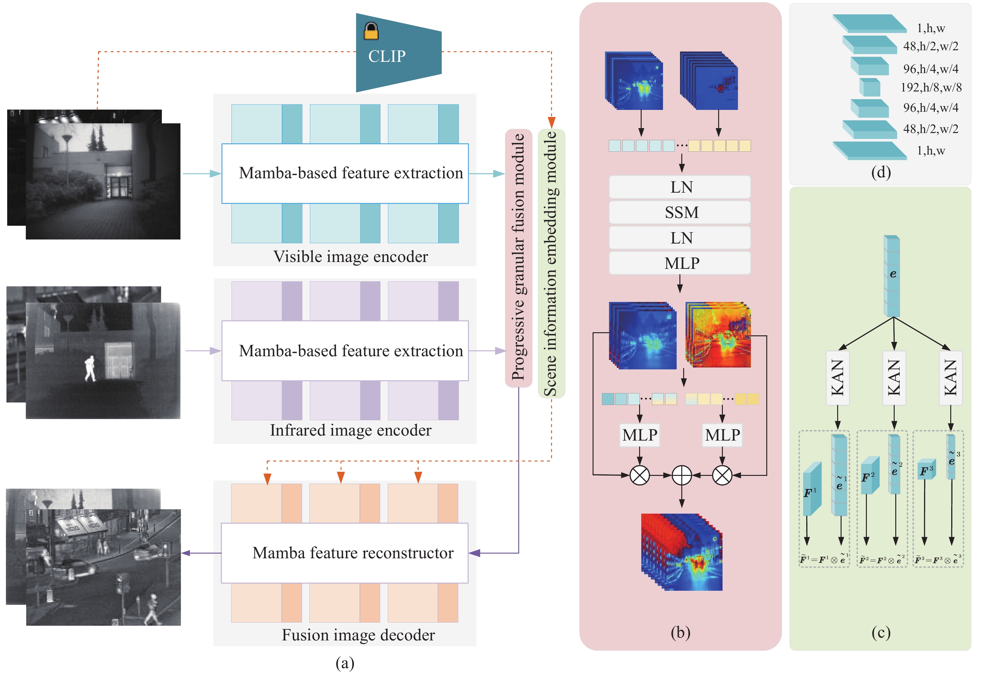
$$ \begin{array}{c}{\widetilde{\boldsymbol{F}}}^{i}={\boldsymbol{F}}^{i}\otimes {\widetilde{\boldsymbol{e}}}^{i}\end{array} $$ (7) 其中,$ {\widetilde{F}}^{i} $和$ {F}^{i} $分别表示嵌入和未嵌入场景编码的融合特征,并且$ {\widetilde{\boldsymbol{F}}}^{i},\;{\boldsymbol{F}}^{i}\in {\mathbf{R}}^{48\times i,h,w} $. 本文通过场景向量来生成逐通道的筛选权重,针对不同的场景,为融合网络中的不同层特征的不同通道赋予不同的权重,从而迫使融合网络可以根据场景信息的不同,自适应地选择合适的特征通道进行融合图像的生成,最终根据场景信息的不同生成不同风格的融合图像. 图1(c)中呈现了所提出场景信息嵌入模块的整体结构,通过CLIP模型得到的场景信息编码被逐层地嵌入到特征提取网络中.
![]() 图 1 整体的网络结构图. (a)整体网络结构; (b)粒度渐进融合模块; (c)场景信息融合模块; (d)特征空间的变化Figure 1. Overall network structure diagram: (a) overall network; (b) Progressive Granular Fusion Module; (c) Scene Information Embedding Module; (d) variation of the feature space
图 1 整体的网络结构图. (a)整体网络结构; (b)粒度渐进融合模块; (c)场景信息融合模块; (d)特征空间的变化Figure 1. Overall network structure diagram: (a) overall network; (b) Progressive Granular Fusion Module; (c) Scene Information Embedding Module; (d) variation of the feature space1.3 粒度渐进融合模块
现有的图像融合方法在处理不同模态的特征时,通常采用精妙设计的模块去融合多模态信息,然而这些方法只在单一的维度上对多模态信息进行处理,忽视了多模态特征在不同特征空间中会表达出了不同特性. 为此,本文提出了一种粒度渐进的融合模块,首先在全局尺度上对多模态特征进行跨空间聚合,接着使用坐标级注意力机制对结构聚合后的特征进行微调. 全局尺度上聚合的过程可以公式化为:
$$ \begin{array}{c}{\boldsymbol{F}}_{G}=G\left(C\right({\boldsymbol{F}}_{\mathrm{v}\mathrm{i}\mathrm{s}},{\boldsymbol{F}}_{\mathrm{i}\mathrm{n}\mathrm{f}})\end{array} $$ (8) 其中,$ {\boldsymbol{F}}_{G} $表示经过全局聚合后的特征,$ G\left(\cdot\right) $运算符为公式4的形式化表示,$ C\left(\cdot\right) $表示沿着通道维度的拼接,$ {\boldsymbol{F}}_{\text{vis}},{\boldsymbol{F}}_{\mathrm{i}\mathrm{n}\mathrm{f}} $分别表示特征提取部分获得的可见光特征和红外特征. 在进行整体聚合后,将聚合特征分离为可见光部分和红外部分,接着使用坐标级注意力机制对其进行微调:
$$ \begin{split} &{\widetilde{\boldsymbol{F}}}_{\mathrm{v}\mathrm{i}\mathrm{s}},{\widetilde{\boldsymbol{F}}}_{\mathrm{i}\mathrm{n}\mathrm{f}}={C}^{-1}\left({\boldsymbol{F}}_{\mathrm{G}}\right)\\ &{\boldsymbol{W}}_{\mathrm{v}\mathrm{i}\mathrm{s}/\mathrm{i}\mathrm{n}\mathrm{f}}=\mathrm{K}\mathrm{A}\mathrm{N}(C\left({\mathrm{M}\mathrm{P}}^{\mathrm{h}}\left({\widetilde{\boldsymbol{F}}}_{\mathrm{v}\mathrm{i}\mathrm{s}}\right),{\mathrm{M}\mathrm{P}}^{w}\left({\widetilde{\boldsymbol{F}}}_{\mathrm{i}\mathrm{n}\mathrm{f}}\right)\right)\\ &{\widetilde{\boldsymbol{W}}}_{\mathrm{v}\mathrm{i}\mathrm{s}/\mathrm{i}\mathrm{n}\mathrm{f}}^{h},{\widetilde{\boldsymbol{W}}}_{\mathrm{v}\mathrm{i}\mathrm{s}/\mathrm{i}\mathrm{n}\mathrm{f}}^{w}={\mathrm{C}}^{-1}\left({\boldsymbol{W}}_{\mathrm{v}\mathrm{i}\mathrm{s}/\mathrm{i}\mathrm{n}\mathrm{f}}\right)\\ &{\boldsymbol{F}}_{\mathrm{f}}={\widetilde{\boldsymbol{F}}}_{\mathrm{v}\mathrm{i}\mathrm{s}}\otimes {\widetilde{\boldsymbol{W}}}_{\mathrm{v}\mathrm{i}\mathrm{s}}^{h}\odot {\widetilde{\boldsymbol{W}}}_{\mathrm{v}\mathrm{i}\mathrm{s}}^{w}+{\widetilde{\boldsymbol{F}}}_{\mathrm{i}\mathrm{n}\mathrm{f}}\otimes {\widetilde{\boldsymbol{W}}}_{\mathrm{i}\mathrm{n}\mathrm{f}}^{h}\odot {\widetilde{\boldsymbol{W}}}_{\mathrm{i}\mathrm{n}\mathrm{f}}^{w}\end{split} $$ (9) 其中,$ {\widetilde{\boldsymbol{F}}}_{\text{vis}},{\widetilde{\boldsymbol{F}}}_{\mathrm{i}\mathrm{n}\mathrm{f}} $表示从全局聚合特征中分离出的可见光特征和红外特征,$ {\mathrm{C}}^{-1}\left(\cdot\right) $表示$ \mathrm{C}\left(\cdot\right) $的逆运算,$ \mathrm{M}{\mathrm{P}}^{\mathrm{h}}\left(\cdot\right),\;\mathrm{M}{\mathrm{P}}^{\mathrm{w}}\left(\cdot\right) $表示沿着h维度和w维度进行最大池化,$ {\boldsymbol{W}}_{\mathrm{v}\mathrm{i}\mathrm{s}/\mathrm{i}\mathrm{n}\mathrm{f}}\in {\mathbf{R}}^{c,h} $表示微调权重,$ {\widetilde{\boldsymbol{W}}}_{\mathrm{v}\mathrm{i}\mathrm{s}/\mathrm{i}\mathrm{n}\mathrm{f}}^{h}\in {\boldsymbol{R}}^{c,h}, {\widetilde{\boldsymbol{W}}}_{\mathrm{v}\mathrm{i}\mathrm{s}/\mathrm{i}\mathrm{n}\mathrm{f}}^{w}\in {\mathbf{R}}^{c,w} $表示h维度和w维度的微调权重,$ \otimes $、$ \odot $分别表示h维度的乘法和w维度的乘法. 通过渐进融合的方式,多模态特征得到多尺度的融合,全局融合是局部融合的前提,局部融合可以弥补全局融合的不足之处.
1.4 整体网络结构
本文所提出融合网络的整体结构如图1(a)所示. 首先,可见光图像和红外图像经过两个不共享参数的特征提取网络进行特征提取;接着,将提取到的特征经过图1(b)所示的粒度渐进融合模块中进行特征融合;然后,融合后的特征和场景感知向量被输入到融合图像解码网络中;最终,得到高质量的融合图像. 对于融合图像解码网络,本文使用了3层连续的基于Mamba的特征处理块进行处理. 对于每层的特征处理块,图像特征在经过特征处理块处理后,利用图1(c)中生成的场景向量,对图像特征进行通道上的调控,完成场景信息的嵌入、融合. 在特征提取的过程中,特征的尺寸不发生改变,通道数逐渐增加,在融合图像重建的过程中,特征通道逐渐减小,直到减小为1即融合图像. 具体的通道数变化情况如图1(d)所示.
1.5 损失函数
首先,使用像素损失、梯度损失和结构相似性损失构建基础的融合损失函数:
$$ \begin{split} &{L}_{\mathrm{b}\mathrm{a}\mathrm{s}\mathrm{e}}(f,{\mathrm{vis}},\mathrm{inf})=\alpha \cdot {\|f-\mathrm{max}(\mathrm{v}\mathrm{i}\mathrm{s},\mathrm{inf})\|}_{1}+\\ &\beta \cdot {\|S\left(f\right)-\mathrm{max}(S\left(\mathrm{v}\mathrm{i}\mathrm{s}\right),S\left(\mathrm{inf})\right)\|}_{1} -\\ &\gamma \cdot \left[\mathrm{S}\mathrm{S}\mathrm{I}\mathrm{M}\right(f,\mathrm{v}\mathrm{i}\mathrm{s})+\mathrm{S}\mathrm{S}\mathrm{I}\mathrm{M}(f,\mathrm{inf})] \end{split}$$ (10) 其中,其中α, β, γ为参数,将在实验部分设置. f、vis、inf分别表示融合图像、可见光图像和红外图像. $ {L}_{\mathrm{b}\mathrm{a}\mathrm{s}\mathrm{e}} $表示基础损失. $ {\|\cdot\|}_{1} $表示1范数,$ \mathrm{max}(\cdot,\cdot) $表示逐原始取大运算,$ S\left(\cdot\right) $表示边缘特征提取,具体的本文使用了Sobel算子执行该运算. $ \mathrm{S}\mathrm{S}\mathrm{I}\mathrm{M}\left(\cdot,\cdot\right) $表示计算两个图像之间的结构相似性. 通过公式(10),融合网络具备了图像融合的能力.
为了让融合网络可以针对不同的场景执行不同的融合任务,公式(10)在训练时被进行调整,当输入场景发生变化,损失对应的进行调节:
$$ \begin{split}&{L}_{\mathrm{f}\mathrm{i}\mathrm{n}\mathrm{a}\mathrm{l}}(f,{\mathrm{vis}},\mathrm{inf})=\theta \cdot {L}_{\mathrm{b}\mathrm{a}\mathrm{s}\mathrm{e}}(f,{\mathrm{vis}},\mathrm{inf})+\\ & (1-\theta )\cdot {L}_{\mathrm{b}\mathrm{a}\mathrm{s}\mathrm{e}}(f,{\mathrm{vi}}{\mathrm{s}}^{\mathrm{h}\mathrm{i}\mathrm{s}\mathrm{t}},{\mathrm{inf}}^{\mathrm{hist}})\end{split} $$ (11) 其中,$ \theta $表示场景选择参数,若当前场景为照明良好的场景,$ \theta $设置为1;场景亮度不佳时,$ \theta $设置为0;$ {L}_{\mathrm{f}\mathrm{i}\mathrm{n}\mathrm{a}\mathrm{l}} $表示所提出网络的总损失. 通过场景选择参数,两个同源异构的损失紧密的联系起来,用以优化多场景融合网络. $ \mathrm{v}\mathrm{i}{\mathrm{s}}^{\mathrm{h}\mathrm{i}\mathrm{s}\mathrm{t}},{\mathrm{i}\mathrm{n}\mathrm{f}}^{\mathrm{h}\mathrm{i}\mathrm{s}\mathrm{t}} $分别表示经过直方图均衡化后的可见光图像和红外图像,由于无监督网络训练难度大,网络难以收敛,采用合理的先验低光增强知识可以降低网络学习的难度. 值得注意的是,网络的输入为未经处理的可见光图像和红外图像,场景亮度的增强依靠网络的学习获得,并不需要额外的计算处理.
2. 实验及结果分析
2.1 实验配置
为了验证所提出方法对红外可见光图像融合效果的有效性,本文将所提出方法和11个最先进的图像融合算法进行比较. 为了公平地对比不同算法之间的性能,在公开数据集MSRS[18],LLVIP[19]和TNO[20]上进行了定量分析和主观分析. 在定量分析中,选取了无参考指标SD、AG、EN和SF用以衡量融合图像的清晰度[21];有参考指标VIF和Qabf用以衡量融合算法的信息整合能力[22]. 其中SD表示图像标准差,其值越大表示融合图像具备更加多样的光影变换. AG表示平均梯度,SF表示空间频率,其值越大表示融合图像具备更加丰富的纹理细节信息. VIF表示视觉保真度,其值越大表示融合图像越符合人眼成像效果. Qabf利用局部度量来估计来自输入的显著信息在融合图像中的表现程度,值越大表示融合图像的信息整合能力越强.
2.2 实施细节
本文代码使用Python进行实现,在Ubuntu20.04上使用Nvidia
3090 进行训练. 训练集为MSRS数据集中选取的1000 对红外图像和可见光图像,并将其裁剪为长宽均为64像素的小块进行训练. 初始学习率设置为0.001,总训练轮次为30,训练至15轮后,每轮学习率衰减为上一轮的0.99. 损失参数$ \alpha ,\;\beta ,\;\gamma $依次设置为50、10和50,计算出梯度后采用Adam优化器对网络参数进行优化.2.3 MSRS数据集上的对比实验
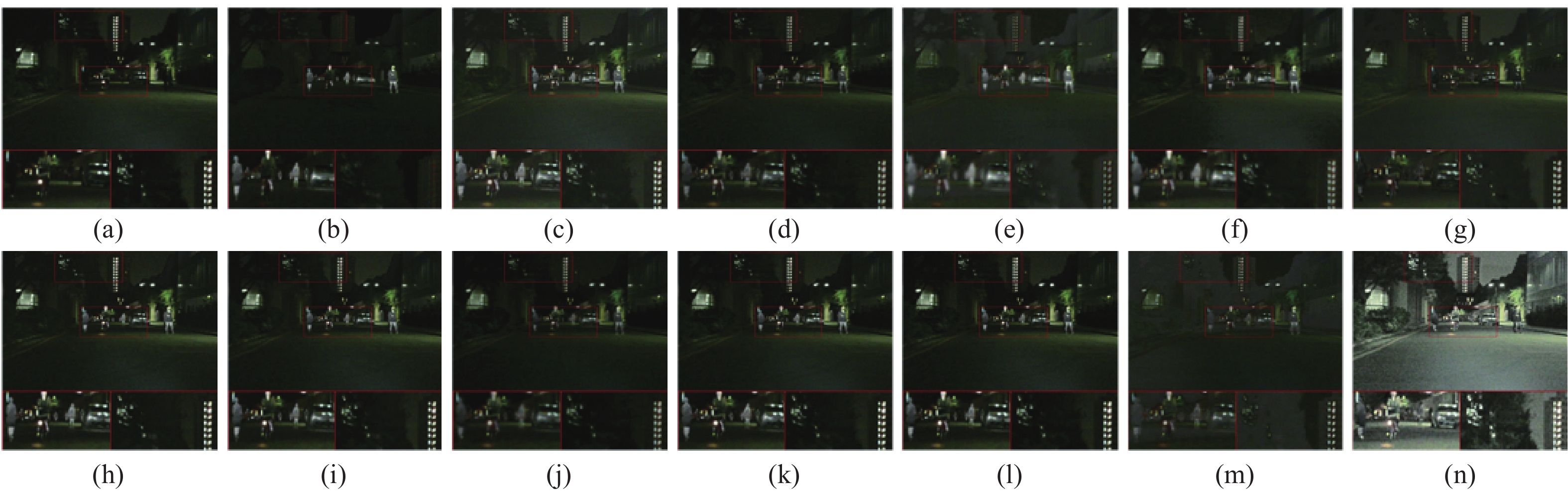
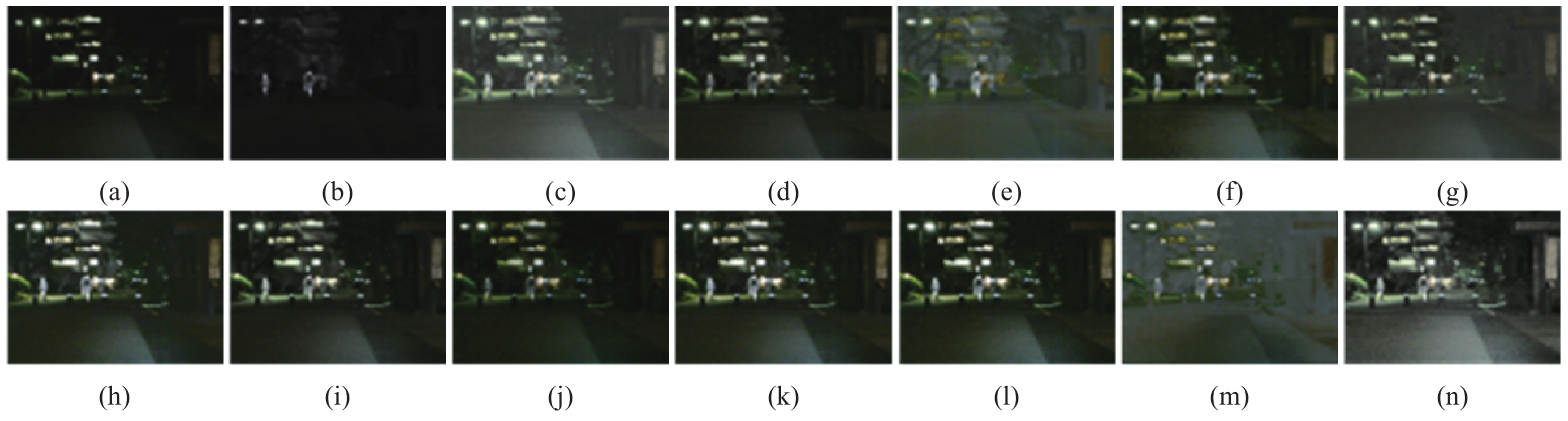
在图2中展示了选取了编号为00750N的图像进行视觉对比的结果. 图2(a)中呈现的可见光图像表明,在亮度极低的夜晚场景下,单一的可见光相机无法很好的反映场景信息. 图2(b)中呈现的红外图像则在各种极端环境下均能稳定地成像,但是缺失了图像的颜色信息和细腻的背景信息,例如远方的高楼. 使用图像融合算法可以利用互补的可见光图像和红外图像生成高质量的融合图像,例如图2(c~m)中的结果,融合图像中既能看到红外图像中的人群信息,又能体现远方的楼房信息. 但是,由于可见光图像亮度极低,导致融合图像的质量依然有限. 对于图像场景中的白色车道线,所有的算法均无法优秀地呈现. 本文方法在应对光线极低的场景时,得益于优秀的场景理解功能,融合网络在执行图像融合任务的同时对场景的亮度进行调节,最终取得的融合图像亮度良好,热辐射清晰,道路车道线边缘锋利.
![]() 图 2 在MSRS数据集上进行定性对比的结果. (a)可见光图像; (b)红外图像; (c) DATFuse生成的图像; (d) DenseFuse生成的图像; (e) FusionGAN生成的图像; (f) GANMcC生成的图像; (g) LRRNet生成的图像; (h) MLFFusion生成的图像; (i) ResCCFusion生成的图像; (j) RFN-Nest生成的图像; (k) SuperFusion生成的图像; (l) SwinFusion生成的图像; (m) UMF-CMGR生成的图像; (n)本文方法生成的图像Figure 2. Results of the qualitative comparison on the MSRS dataset: (a) the visible image; (b) the infrared image; (c) the image generated by DATFuse; (d) the image generated by DenseFuse; (e) the image generated by FusionGAN; (f) the image generated by GANMcC; (g) the image generated by LRRNet; (h) the image generated by MLFFusion; (i) the image generated by ResCCFusion; (j) the image generated by RFN-Nest; (k) the image generated by SuperFusion; (l) the image generated by SwinFusion; (m) the image generated by UMF-CMGR; (n) the image generated by the proposed method
图 2 在MSRS数据集上进行定性对比的结果. (a)可见光图像; (b)红外图像; (c) DATFuse生成的图像; (d) DenseFuse生成的图像; (e) FusionGAN生成的图像; (f) GANMcC生成的图像; (g) LRRNet生成的图像; (h) MLFFusion生成的图像; (i) ResCCFusion生成的图像; (j) RFN-Nest生成的图像; (k) SuperFusion生成的图像; (l) SwinFusion生成的图像; (m) UMF-CMGR生成的图像; (n)本文方法生成的图像Figure 2. Results of the qualitative comparison on the MSRS dataset: (a) the visible image; (b) the infrared image; (c) the image generated by DATFuse; (d) the image generated by DenseFuse; (e) the image generated by FusionGAN; (f) the image generated by GANMcC; (g) the image generated by LRRNet; (h) the image generated by MLFFusion; (i) the image generated by ResCCFusion; (j) the image generated by RFN-Nest; (k) the image generated by SuperFusion; (l) the image generated by SwinFusion; (m) the image generated by UMF-CMGR; (n) the image generated by the proposed method为了定量地将本文方法与这些最先进的方法进行对比分析,表1中展示了对实验情况进行定量对比的结果. 得益于本文方法对场景亮度的自适应调节能力,本文方法在SD、VIF、AG、EN和SF的对比上均取得了较为显著的优势. 然而,亮度调节在改善融合图像视觉效果的同时,也拉大了结果和原始低质量可见光之间的距离,因此,Qabf指标体现出相对偏低的情况.
表 1 在MSRS数据集上的定量对比Table 1. Quantitative comparison on the MSRS datasetsMethod Year SD VIF AG EN Qabf SF DenseFuse[9] 2019 21.7389 0.7632 1.8535 5.5269 0.4382 5.6679 FusionGAN[13] 2019 17.1449 0.4132 1.2088 5.2505 0.1382 3.8752 GANMcC[12] 2021 24.3486 0.6825 1.8351 5.8325 0.3384 5.2267 RFN-Nest[10] 2021 21.5879 0.5741 1.2661 5.3887 0.2417 4.3374 SuperFusion[23] 2022 32.1587 0.9169 2.5704 5.9026 0.5886 8.5035 SwinFusion[17] 2022 32.8862 0.9570 2.6751 5.9138 0.5806 8.7782 UMF-CMGR[24] 2022 16.8892 0.3084 1.7376 5.0580 0.2320 6.0331 LRRNet[25] 2023 20.3234 0.4362 1.6918 5.1835 0.3084 6.0885 DATFuse[26] 2023 27.0892 0.8493 2.6178 5.8089 0.5418 8.8730 ResCCFusion[27] 2024 29.8823 0.9416 2.5002 5.8360 0.6294 8.3571 MLFFusion[28] 2023 33.3281 0.9769 3.0618 5.8053 0.6311 9.6072 Ours 47.8841 1.2566 6.0620 7.2697 0.3043 15.6929 2.4 TNO数据集上的对比实验
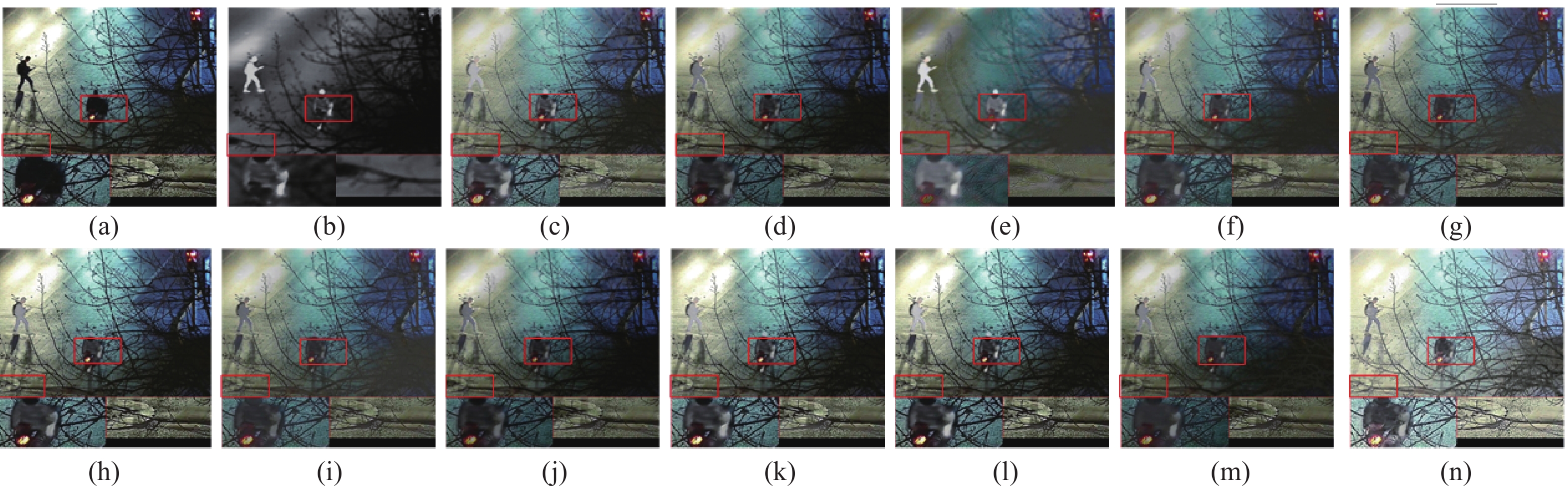
为了展示本文模型在不同场景下的强大泛化能力,本文在光照正常的TNO数据集上再次进行了实验. 图3中展示了本文方法与最先进的融合算法在TNO数据集上的融合效果对比. 可见光无法呈现隐藏在黑暗中的人物信息,红外图像无法呈现细腻的背景信息. (c)(k)图像整体较为模糊. (e)(f)两种基于GAN的方法出现了严重的亮度退化. (g)(h)(j)方法融合不充分,人物的热辐射信息在融合过程中被减弱. 剩余几种方法和本文方法均取得了较好的融合效果,但是相比之下,本文方法的人物具备更加锐利的边缘.
![]() 图 3 在TNO数据集上进行定性对比的结果. (a)可见光图像; (b)红外图像; (c) DATFuse生成的图像; (d) DenseFuse生成的图像; (e) FusionGAN生成的图像; (f) GANMcC生成的图像; (g) LRRNet生成的图像; (h) MLFFusion生成的图像; (i) ResCCFusion生成的图像; (j) RFN-Nest生成的图像; (k) SuperFusion生成的图像; (l) SwinFusion生成的图像; (m) UMF-CMGR生成的图像; (n)本文方法生成的图像Figure 3. Results of the qualitative comparison on the TNO dataset: (a) the visible image; (b) the infrared image; (c) the image generated by DATFuse; (d) the image generated by DenseFuse; (e) the image generated by FusionGAN; (f) the image generated by GANMcC; (g) the image generated by LRRNet; (h) the image generated by MLFFusion; (i) the image generated by ResCCFusion; (j) the image generated by RFN-Nest; (k) the image generated by SuperFusion; (l) the image generated by SwinFusion; (m) the image generated by UMF-CMGR; (n) the image generated by the proposed method
图 3 在TNO数据集上进行定性对比的结果. (a)可见光图像; (b)红外图像; (c) DATFuse生成的图像; (d) DenseFuse生成的图像; (e) FusionGAN生成的图像; (f) GANMcC生成的图像; (g) LRRNet生成的图像; (h) MLFFusion生成的图像; (i) ResCCFusion生成的图像; (j) RFN-Nest生成的图像; (k) SuperFusion生成的图像; (l) SwinFusion生成的图像; (m) UMF-CMGR生成的图像; (n)本文方法生成的图像Figure 3. Results of the qualitative comparison on the TNO dataset: (a) the visible image; (b) the infrared image; (c) the image generated by DATFuse; (d) the image generated by DenseFuse; (e) the image generated by FusionGAN; (f) the image generated by GANMcC; (g) the image generated by LRRNet; (h) the image generated by MLFFusion; (i) the image generated by ResCCFusion; (j) the image generated by RFN-Nest; (k) the image generated by SuperFusion; (l) the image generated by SwinFusion; (m) the image generated by UMF-CMGR; (n) the image generated by the proposed method为了进一步说明本文方法的有效性,表2中展示了本文方法和对比方法在TNO数据集上的定量对比. 与视觉对比相对应,本文方法的AG、SF取得了最佳的结果,表明本文方法生成的融合图像具备良好的纹理细节信息. 在Qabf的对比上,本文方法的指标依然位列前茅, 证明本文方法具备强大的信息整合能力. 但是本文方法的SD、VIF和EN有着轻微的落后,这是由于本文方法并没有将过多的提升重点放在单个图像指标的轻微提升上,而是重在设计适应多场景的图像融合网络.
表 2 在TNO数据集上的定量对比Table 2. Quantitative comparison on the TNO datasetsMethod SD VIF AG EN Qabf SF DenseFuse[9] 34.8425 0.6630 3.5432 6.8206 0.4471 8.9475 FusionGAN[13] 30.7810 0.4244 2.4184 6.5572 0.2343 6.2719 GANMcC[12] 33.4233 0.5324 2.5204 6.7338 0.2787 6.1114 RFN-Nest[10] 36.9403 0.5614 2.6541 6.9661 0.3334 5.8461 SuperFusion[23] 37.0824 0.6858 3.5658 6.7629 0.4757 9.2355 SwinFusion[17] 39.7786 0.7651 4.2170 6.9082 0.5261 10.7610 UMF-CMGR[24] 30.1167 0.5981 2.9691 6.5371 0.4114 8.1779 LRRNet[25] 40.9867 0.5636 3.7621 6.9909 0.3533 9.5100 DATFuse[26] 28.3505 0.7301 3.6975 6.5507 0.5227 10.0466 ResCCFusion[27] 40.7118 0.8277 3.8048 7.0003 0.5195 10.0035 MLFFusion[28] 41.4123 0.7548 4.0195 6.9071 0.5192 10.0094 Ours 39.5807 0.6670 4.5763 6.9438 0.5265 11.9243 2.5 LLVIP数据集上的实验
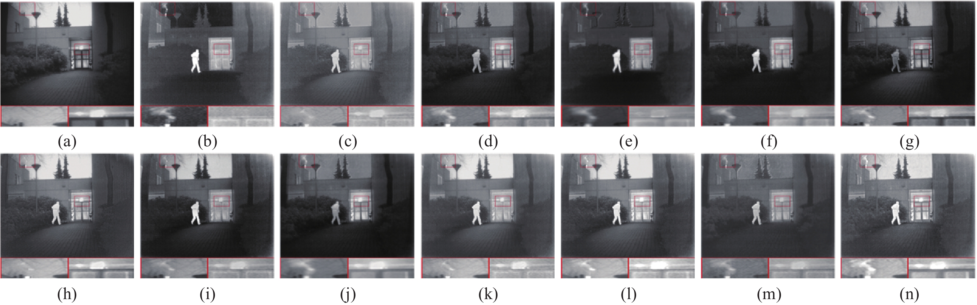
为了验证本文方法的泛化能力,从LLVIP数据集上依旧选取了图像进行视觉效果的对比. 图4中呈现了对比的结果. 可见光图像并没有出现极端黑暗的场景,因此几种图像融合方法都取得了视觉效果良好的融合图像. 然而对于局部的黑暗区域,例如放大区域的井盖和行人,常规的图像融合方法并不能很好地勾勒出物体的纹理边缘,得益于本文方法具备文本引导的亮度调节功能,黑暗的井盖区域纹理清晰,隐藏在黑暗中的行人也无所遁形.
![]() 图 4 在LLVIP数据集上进行定性对比的结果. (a)可见光图像; (b)红外图像; (c) DATFuse生成的图像; (d) DenseFuse生成的图像; (e) FusionGAN生成的图像; (f) GANMcC生成的图像; (g) LRRNet生成的图像; (h) MLFFusion生成的图像; (i) ResCCFusion生成的图像; (j) RFN-Nest生成的图像; (k) SuperFusion生成的图像; (l) SwinFusion生成的图像; (m) UMF-CMGR生成的图像; (n)本文方法生成的图像Figure 4. Results of the qualitative comparisons on the LLVIP dataset: (a) the visible image; (b) the infrared image; (c) the image generated by DATFuse; (d) the image generated by DenseFuse; (e) the image generated by FusionGAN; (f) the image generated by GANMcC; (g) the image generated by LRRNet; (h) the image generated by MLFFusion; (i) the image generated by ResCCFusion; (j) the image generated by RFN-Nest; (k) the image generated by SuperFusion; (l) the image generated by SwinFusion; (m) the image generated by UMF-CMGR; (n) the image generated by the proposed method
图 4 在LLVIP数据集上进行定性对比的结果. (a)可见光图像; (b)红外图像; (c) DATFuse生成的图像; (d) DenseFuse生成的图像; (e) FusionGAN生成的图像; (f) GANMcC生成的图像; (g) LRRNet生成的图像; (h) MLFFusion生成的图像; (i) ResCCFusion生成的图像; (j) RFN-Nest生成的图像; (k) SuperFusion生成的图像; (l) SwinFusion生成的图像; (m) UMF-CMGR生成的图像; (n)本文方法生成的图像Figure 4. Results of the qualitative comparisons on the LLVIP dataset: (a) the visible image; (b) the infrared image; (c) the image generated by DATFuse; (d) the image generated by DenseFuse; (e) the image generated by FusionGAN; (f) the image generated by GANMcC; (g) the image generated by LRRNet; (h) the image generated by MLFFusion; (i) the image generated by ResCCFusion; (j) the image generated by RFN-Nest; (k) the image generated by SuperFusion; (l) the image generated by SwinFusion; (m) the image generated by UMF-CMGR; (n) the image generated by the proposed method为了定量地对比,表3呈现了指标对比的结果. MLFFusion配备了具备亮度保持功能的损失函数,导致其在亮度较差的环境中表现较好. 在VIF,AG,EN,SF的对比上,本文方法取得了最佳结果. 和MSRS数据集上的结果类似,亮度调节导致Qabf的下降,这种下降并不能说明本文方法不具备良好的信息整合能力.
表 3 在LLVIP数据集上的定量对比Table 3. Quantitative comparison on the LLVIP datasetsMethod SD VIF AG EN Qabf SF DenseFuse[9] 34.1926 0.7669 2.7220 6.8751 0.4885 9.2664 FusionGAN[13] 24.8206 0.4762 1.9468 6.3083 0.2539 6.9194 GANMcC[12] 32.1132 0.6125 2.1229 6.6899 0.2972 6.8144 RFN-Nest[10] 34.6463 0.6693 2.1579 6.8624 0.3129 6.3211 SuperFusion[23] 42.3495 0.8180 3.1196 7.1280 0.5281 11.1390 SwinFusion[17] 44.9182 0.9324 3.9154 7.1586 0.6489 13.6233 UMF-CMGR[24] 29.3794 0.5208 2.5041 6.4620 0.3473 9.9154 LRRNet[25] 24.8671 0.5640 2.4671 6.1452 0.4242 9.1082 DATFuse[26] 39.8505 0.8388 3.0364 7.0820 0.5136 12.3311 ResCCFusion[27] 24.8671 0.5640 2.4671 6.1452 0.4242 9.1082 MLFFusion[28] 46.5614 0.9596 4.0846 7.2267 0.6751 13.9526 Ours 43.5546 1.0832 7.5902 7.3343 0.3263 23.1897 2.6 雾霾场景下的实验
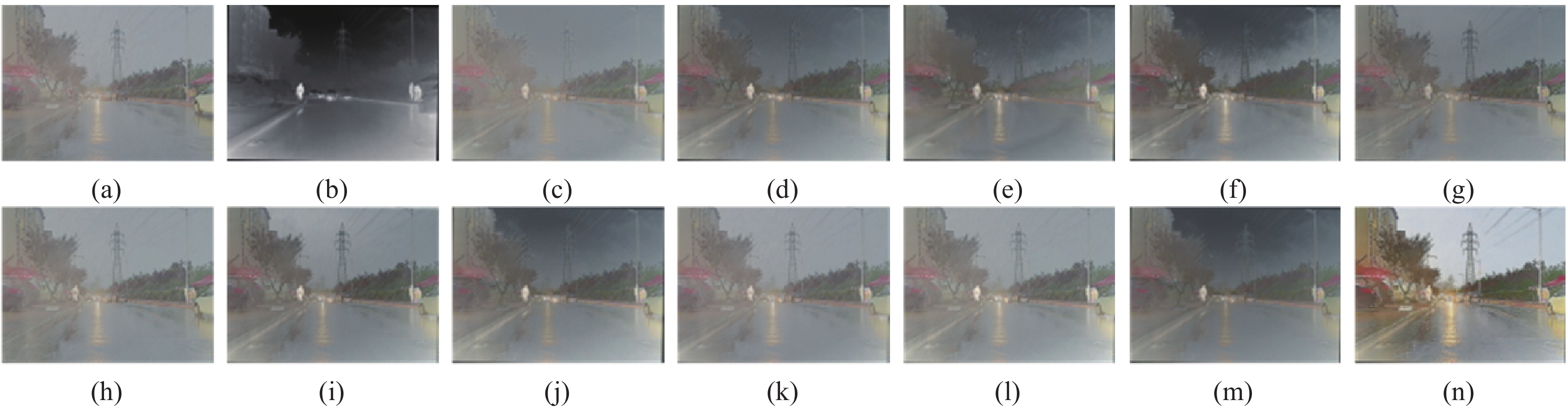
为了验证所提出方法在极端气候下的稳定性,图5从M3FD数据集中选择了一对典型的图像进行视觉效果对比,呈现了不同方法在雾霾环境下的效果. 对于不同的对比方法,在雾霾环境下不可避免地出现了画面模糊的问题,尽管DenseFuse,FusionGAN,GANMcC,RFN-Nest和UMF-CMGR依靠着强大的信息选择能力使用红外信息对雾霾干扰进行了抑制,但是整体的场景亮度出现了明显的退化. 借助于大模型的场景信息嵌入,本文方法在雾霾环境下依旧取得了较为优秀的视觉效果.
![]() 图 5 在M3FD数据集上进行定性对比的结果. (a)可见光图像; (b)红外图像; (c) DATFuse生成的图像; (d) DenseFuse生成的图像; (e) FusionGAN生成的图像; (f) GANMcC生成的图像; (g) LRRNet生成的图像; (h) MLFFusion生成的图像; (i) ResCCFusion生成的图像; (j) RFN-Nest生成的图像; (k) SuperFusion生成的图像; (l) SwinFusion生成的图像; (m) UMF-CMGR生成的图像; (n)本文方法生成的图像Figure 5. Results of the qualitative comparisons on the M3FD dataset: (a) the visible image; (b) the infrared image; (c) the image generated by DATFuse; (d) the image generated by DenseFuse; (e) the image generated by FusionGAN; (f) the image generated by GANMcC; (g) the image generated by LRRNet; (h) the image generated by MLFFusion; (i) the image generated by ResCCFusion; (j) the image generated by RFN-Nest; (k) the image generated by SuperFusion; (l) the image generated by SwinFusion; (m) the image generated by UMF-CMGR; (n) the image generated by the proposed method
图 5 在M3FD数据集上进行定性对比的结果. (a)可见光图像; (b)红外图像; (c) DATFuse生成的图像; (d) DenseFuse生成的图像; (e) FusionGAN生成的图像; (f) GANMcC生成的图像; (g) LRRNet生成的图像; (h) MLFFusion生成的图像; (i) ResCCFusion生成的图像; (j) RFN-Nest生成的图像; (k) SuperFusion生成的图像; (l) SwinFusion生成的图像; (m) UMF-CMGR生成的图像; (n)本文方法生成的图像Figure 5. Results of the qualitative comparisons on the M3FD dataset: (a) the visible image; (b) the infrared image; (c) the image generated by DATFuse; (d) the image generated by DenseFuse; (e) the image generated by FusionGAN; (f) the image generated by GANMcC; (g) the image generated by LRRNet; (h) the image generated by MLFFusion; (i) the image generated by ResCCFusion; (j) the image generated by RFN-Nest; (k) the image generated by SuperFusion; (l) the image generated by SwinFusion; (m) the image generated by UMF-CMGR; (n) the image generated by the proposed method为了客观地分析所提出方法在雾霾环境下的性能,本文从M3FD数据集中选取了10对雾霾图像,使用不同的融合方法得到融合结果,表4呈现了定量指标的对比. 得益于基于大模型的语义信息注入,本文方法在SD、VIF、AG、EN和SF的对比上均取得了较好的水平.
表 4 在M3FD定量对比Table 4. Quantitative comparison on the M3FD datasetsMethod SD VIF AG EN Qabf SF DenseFuse[9] 26.1373 0.7985 2.3549 6.6033 0.5199 7.1329 FusionGAN[13] 27.8432 0.5656 2.3499 6.7448 0.3377 6.6424 GANMcC[12] 30.4889 0.5040 1.9505 6.8846 0.2841 5.5501 RFN-Nest[10] 32.1853 0.6962 2.0794 6.9956 0.4214 5.7635 SuperFusion[23] 17.7198 0.8197 2.2826 5.9919 0.5455 7.1204 SwinFusion[17] 19.0168 0.8721 2.5661 6.0927 0.5638 7.8699 UMF-CMGR[24] 24.0267 0.6658 1.7974 6.5609 0.3735 5.6679 LRRNet[25] 19.4493 0.6445 2.6237 6.2279 0.4695 8.3066 DATFuse[26] 13.4647 0.6995 2.5456 5.6910 0.5116 7.9709 ResCCFusion[27] 25.0947 0.6918 2.9221 6.6176 0.4440 9.0550 MLFFusion[28] 17.4232 0.9546 2.5260 5.9499 0.6028 7.9004 Ours 47.0762 0.7902 5.2970 7.0008 0.3046 16.5346 2.7 动态场景下的实验
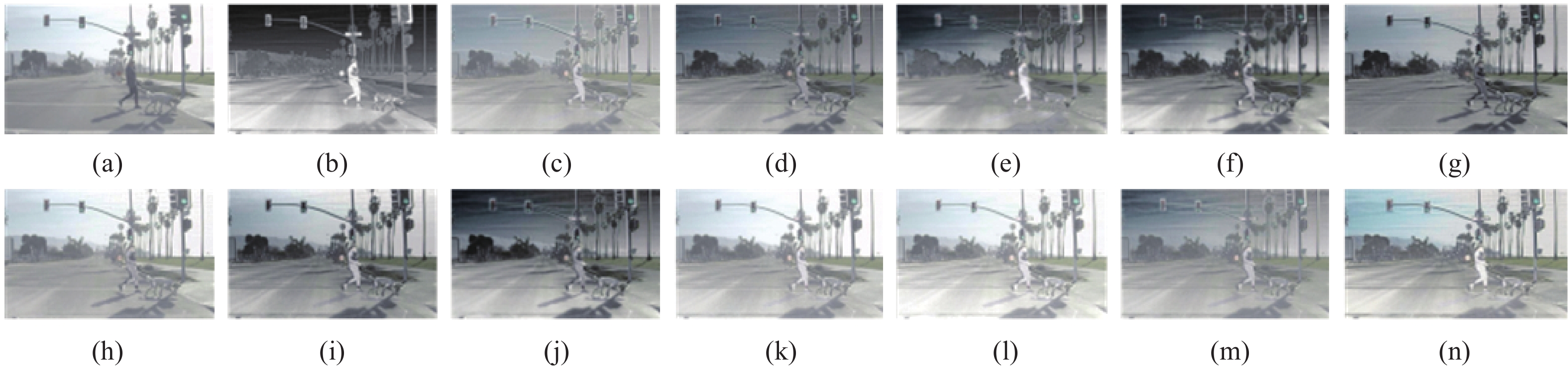
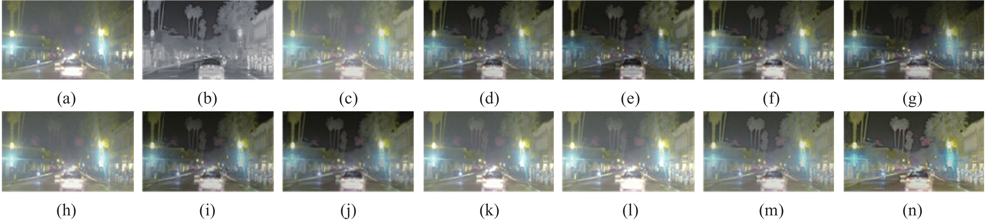
为了进一步验证所提出算法在动态场景下的泛化能力,本文从RoadScene数据集中选取了两个连续的场景,分别为日间的路口和夜间的路口,并在图6和图7中展示了定性对比的结果. 图6展示了在日间环境下的融合结果,本文方法正确地识别到当前的场景信息,实现了精准的图像融合任务. 图7展示了在夜间环境下的融合结果,本文方法在融合的过程中对亮度进行了微调,夜间的炫光被得到了抑制.
![]() 图 6 在RoadScene数据集上选取日间环境进行定性对比的结果. (a)可见光图像; (b)红外图像; (c) DATFuse生成的图像; (d) DenseFuse生成的图像; (e) FusionGAN生成的图像; (f) GANMcC生成的图像; (g) LRRNet生成的图像; (h) MLFFusion生成的图像; (i) ResCCFusion生成的图像; (j) RFN-Nest生成的图像; (k) SuperFusion生成的图像; (l) SwinFusion生成的图像; (m) UMF-CMGR生成的图像; (n)本文方法生成的图像Figure 6. Results of the qualitative comparisons on the RoadScene dataset in daytime: (a) the visible image; (b) the infrared image; (c) the image generated by DATFuse; (d) the image generated by DenseFuse; (e) the image generated by FusionGAN; (f) the image generated by GANMcC; (g) the image generated by LRRNet; (h) the image generated by MLFFusion; (i) the image generated by ResCCFusion; (j) the image generated by RFN-Nest; (k) the image generated by SuperFusion; (l) the image generated by SwinFusion; (m) the image generated by UMF-CMGR; (n) the image generated by the proposed method
图 6 在RoadScene数据集上选取日间环境进行定性对比的结果. (a)可见光图像; (b)红外图像; (c) DATFuse生成的图像; (d) DenseFuse生成的图像; (e) FusionGAN生成的图像; (f) GANMcC生成的图像; (g) LRRNet生成的图像; (h) MLFFusion生成的图像; (i) ResCCFusion生成的图像; (j) RFN-Nest生成的图像; (k) SuperFusion生成的图像; (l) SwinFusion生成的图像; (m) UMF-CMGR生成的图像; (n)本文方法生成的图像Figure 6. Results of the qualitative comparisons on the RoadScene dataset in daytime: (a) the visible image; (b) the infrared image; (c) the image generated by DATFuse; (d) the image generated by DenseFuse; (e) the image generated by FusionGAN; (f) the image generated by GANMcC; (g) the image generated by LRRNet; (h) the image generated by MLFFusion; (i) the image generated by ResCCFusion; (j) the image generated by RFN-Nest; (k) the image generated by SuperFusion; (l) the image generated by SwinFusion; (m) the image generated by UMF-CMGR; (n) the image generated by the proposed method![]() 图 7 在RoadScene数据集上选取夜间环境进行定性对比的结果(a)可见光图像; (b)红外图像; (c) DATFuse生成的图像; (d) DenseFuse生成的图像; (e) FusionGAN生成的图像; (f) GANMcC生成的图像; (g) LRRNet生成的图像; (h) MLFFusion生成的图像; (i) ResCCFusion生成的图像; (j) RFN-Nest生成的图像; (k) SuperFusion生成的图像; (l) SwinFusion生成的图像; (m) UMF-CMGR生成的图像; (n)本文方法生成的图像Figure 7. Results of the qualitative comparisons on theRoadScene dataset in nighttime: (a) the visible image; (b) the infrared image; (c) the image generated by DATFuse; (d) the image generated by DenseFuse; (e) the image generated by FusionGAN; (f) the image generated by GANMcC; (g) the image generated by LRRNet; (h) the image generated by MLFFusion; (i) the image generated by ResCCFusion; (j) the image generated by RFN-Nest; (k) the image generated by SuperFusion; (l) the image generated by SwinFusion; (m) the image generated by UMF-CMGR; (n) the image generated by the proposed method
图 7 在RoadScene数据集上选取夜间环境进行定性对比的结果(a)可见光图像; (b)红外图像; (c) DATFuse生成的图像; (d) DenseFuse生成的图像; (e) FusionGAN生成的图像; (f) GANMcC生成的图像; (g) LRRNet生成的图像; (h) MLFFusion生成的图像; (i) ResCCFusion生成的图像; (j) RFN-Nest生成的图像; (k) SuperFusion生成的图像; (l) SwinFusion生成的图像; (m) UMF-CMGR生成的图像; (n)本文方法生成的图像Figure 7. Results of the qualitative comparisons on theRoadScene dataset in nighttime: (a) the visible image; (b) the infrared image; (c) the image generated by DATFuse; (d) the image generated by DenseFuse; (e) the image generated by FusionGAN; (f) the image generated by GANMcC; (g) the image generated by LRRNet; (h) the image generated by MLFFusion; (i) the image generated by ResCCFusion; (j) the image generated by RFN-Nest; (k) the image generated by SuperFusion; (l) the image generated by SwinFusion; (m) the image generated by UMF-CMGR; (n) the image generated by the proposed method为了客观地评价所提出方法在动态场景下的泛化能力,本文从RoadScene数据集中选取了40对图像,这40对图像分别是不同时间段的道路环境,并统计了不同融合算法获得的定量指标,呈现在表5中. 表5中的数据表明,在极具挑战性的动态场景下,本文方法在VIF、AG、Qabf和SF上依旧取得了最佳的效果. 尽管ResCCFusion在SD和EN上取得了更好的结果,但是综合地对指标进行分析发现本文方法取得了更加均衡的效果. 所提出方法在动态场景下的鲁棒性得到了验证.
表 5 在RoadScene定量对比Table 5. Quantitative comparison on the RoadScene datasetsMethod SD VIF AG EN Qabf SF DenseFuse[9] 41.6418 0.5663 5.1588 7.2664 0.4679 13.3948 FusionGAN[13] 38.6246 0.3528 3.5230 7.0938 0.2573 9.0313 GANMcC[12] 44.3764 0.4776 4.0184 7.3113 0.3286 9.4598 RFN-Nest[10] 45.6429 0.4871 3.7070 7.3672 0.3104 8.6350 SuperFusion[23] 42.2997 0.5884 4.7654 7.0008 0.4459 13.0590 SwinFusion[17] 44.5553 0.5879 4.8509 7.0231 0.4379 12.9205 UMF-CMGR[24] 35.2428 0.5478 4.6126 7.0400 0.4427 12.0836 LRRNet[25] 43.3252 0.4882 5.0379 7.1686 0.3602 13.3470 DATFuse[26] 29.9707 0.5481 4.3028 6.7718 0.4439 12.0730 ResCCFusion[27] 50.5523 0.6253 5.3980 7.4612 0.4914 14.2099 MLFFusion[28] 41.9363 0.6863 4.5580 7.0460 0.4614 13.0562 Ours 46.7927 0.7513 6.5371 7.3818 0.6184 17.2539 2.8 级联方法的对比
在夜间环境下,本文方法可以在图像融合的过程中执行低光增强任务. 为了证明所提出方法在视觉效果和定量指标的对比上要优于先增强、后融合的方法,本文在MSRS数据集上先使用SCI[16]算法对暗光的可见光图像进行亮度增强,接着使用不同的融合算法对增强后的可见光和红外图像进行融合,图8呈现了先增强、后融合的视觉效果对比. 可以看到,级联的方式在提升图像亮度的同时,也错误地放大了黑暗图像中的噪声信息,并且级联的方式所获得的场景亮度要低于本文方法.
![]() 图 8 在MSRS数据集上级联方法进行定性对比的结果 (a)可见光图像; (b)红外图像; (c) DATFuse生成的图像; (d) DenseFuse生成的图像; (e) FusionGAN生成的图像; (f) GANMcC生成的图像; (g) LRRNet生成的图像; (h) MLFFusion生成的图像; (i) ResCCFusion生成的图像; (j) RFN-Nest生成的图像; (k) SuperFusion生成的图像; (l) SwinFusion生成的图像; (m) UMF-CMGR生成的图像; (n)本文方法生成的图像Figure 8. Results of the qualitative comparisons of cascade methods on the MSRS dataset: (a) the visible image; (b) the infrared image; (c) the image generated by DATFuse; (d) the image generated by DenseFuse; (e) the image generated by FusionGAN; (f) the image generated by GANMcC; (g) the image generated by LRRNet; (h) the image generated by MLFFusion; (i) the image generated by ResCCFusion; (j) the image generated by RFN-Nest; (k) the image generated by SuperFusion; (l) the image generated by SwinFusion; (m) the image generated by UMF-CMGR; (n) the image generated by the proposed method
图 8 在MSRS数据集上级联方法进行定性对比的结果 (a)可见光图像; (b)红外图像; (c) DATFuse生成的图像; (d) DenseFuse生成的图像; (e) FusionGAN生成的图像; (f) GANMcC生成的图像; (g) LRRNet生成的图像; (h) MLFFusion生成的图像; (i) ResCCFusion生成的图像; (j) RFN-Nest生成的图像; (k) SuperFusion生成的图像; (l) SwinFusion生成的图像; (m) UMF-CMGR生成的图像; (n)本文方法生成的图像Figure 8. Results of the qualitative comparisons of cascade methods on the MSRS dataset: (a) the visible image; (b) the infrared image; (c) the image generated by DATFuse; (d) the image generated by DenseFuse; (e) the image generated by FusionGAN; (f) the image generated by GANMcC; (g) the image generated by LRRNet; (h) the image generated by MLFFusion; (i) the image generated by ResCCFusion; (j) the image generated by RFN-Nest; (k) the image generated by SuperFusion; (l) the image generated by SwinFusion; (m) the image generated by UMF-CMGR; (n) the image generated by the proposed method表6中呈现了级联方法与本文方法的定量指标对比. 经过亮度增强算法进行增强后,由于融合图像的质量得到改善,因此不同方法的指标值相比于直接融合均有提升. 尽管如此,本文方法在SD、VIF、AG、EN和SF的对比上依旧取得了最佳的效果. 由于本文方法在融合的过程中充分地增强了场景的亮度,因此融合图像和可见光图像之间的相似度变低,从而导致本文方法在Qabf的对比上没有取得最佳的水平.
表 6 在MSRS数据集上级联方法的定量指标对比Table 6. Comparison of quantitative metrics for cascade methods on the MSRS datasetMethod SD VIF AG EN Qabf SF DenseFuse[9] 36.3769 1.0095 3.5126 5.9035 0.5453 9.6305 FusionGAN[13] 26.7274 0.5313 2.1367 6.1548 0.2406 6.2425 GANMcC[12] 39.6900 0.8603 3.3213 6.7057 0.4334 8.4948 RFN-Nest[10] 36.1940 0.7463 2.2290 6.3065 0.3672 6.8413 SuperFusion[23] 45.4127 1.0689 4.3345 6.7453 0.4551 11.9034 SwinFusion[17] 46.5278 1.0874 4.4845 6.7618 0.4247 12.3741 UMF-CMGR[24] 25.1042 0.3768 3.1528 6.0111 0.3112 9.1723 LRRNet[25] 31.5402 0.5071 3.0804 5.5901 0.3694 9.8270 DATFuse[26] 39.3817 1.0232 4.4120 6.2832 0.3636 13.0349 MLFFusion[27] 45.7913 1.0994 5.2045 6.6393 0.3541 13.8107 ResCCFusion[28] 43.7759 1.2038 4.3400 6.2440 0.4877 12.3908 Ours 47.8841 1.2566 6.0620 7.2697 0.3043 15.6929 2.9 消融实验
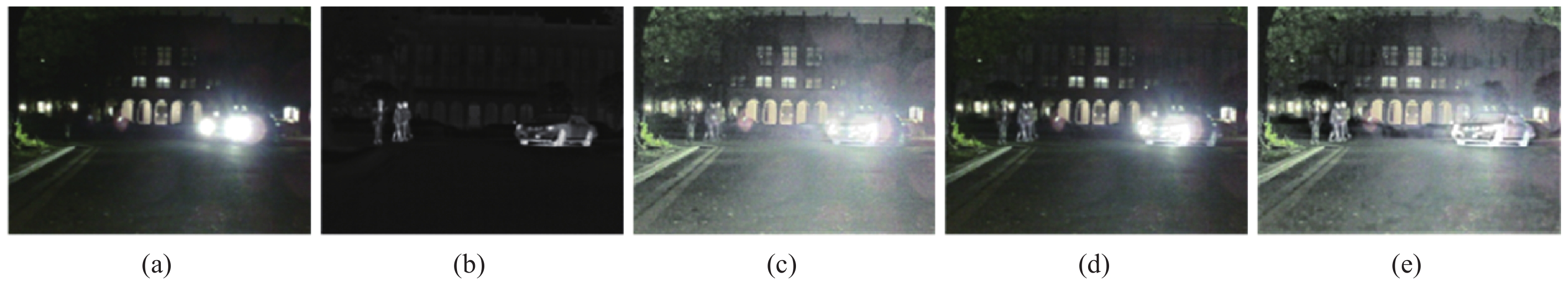
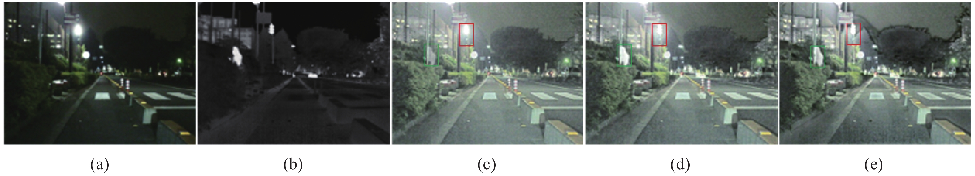
为了证明所提出模块的有效性,本文依次从网络中移除场景信息嵌入模块和粒度渐进模块,在MSRS数据集上开展了针对所提出模块的消融实验. 移除后的视觉对比结果如图9所示. 当移除粒度渐进融合模块后,经过增强的、差异较大的多模态特征无法得到充分的融合,导致具备融合难度的车灯区域成像不佳. 当移除场景信息感知模块后,让融合网络无法充分地理解场景信息,从而导致黑暗场景下的图像没有得到充分的增强. 得益于所提出模块的有效性,本文方法对场景理解正确,图像融合充分,融合图像视觉效果较好. 表7中呈现了针对模块的消融实验的定量对比结果. 数据表明,在嵌入所提出模块后,融合网络达到了最佳性能,模块的有效性被再次得到证明.
![]() 图 9 模块消融实验对比效果图. (a)可见光图像;(b)红外图像;(c)移除粒度渐进融合模块后生成的融合图像;(d)移除场景信息感知模块后生成的融合图像;(e)本文方法生成的融合图像.Figure 9. Visual contrast rendering of the module ablation experiment: (a)the visible light image; (b) the infrared image; (c) the fused image generated after removing the granularity-progressive fusion module; (d) the fused image generated after removing the scene information perception module; (e) the fused image generated by the proposed method.表 7 模块消融实验的定量对比Table 7. Quantitative comparison of module ablation experiments.
图 9 模块消融实验对比效果图. (a)可见光图像;(b)红外图像;(c)移除粒度渐进融合模块后生成的融合图像;(d)移除场景信息感知模块后生成的融合图像;(e)本文方法生成的融合图像.Figure 9. Visual contrast rendering of the module ablation experiment: (a)the visible light image; (b) the infrared image; (c) the fused image generated after removing the granularity-progressive fusion module; (d) the fused image generated after removing the scene information perception module; (e) the fused image generated by the proposed method.表 7 模块消融实验的定量对比Table 7. Quantitative comparison of module ablation experiments.Method SD VIF AG EN Qabf SF A 46.3691 1.2097 5.0382 7.1851 0.2812 13.716 B 34.8423 0.9917 3.5474 6.4095 0.5463 10.105 Ours 47.8841 1.2566 6.0620 7.2697 0.3043 15.6929 Notes:A represents the network with the granularity-progressive fusion module removed, and B represents the network with the scene information perception module removed 本文的特征提取部分是基于状态空间方程进行设计,为了证明本文所提出的特征提取模块要优于现有的主流特征提取器Transformer和CNN,本文对特征提取模块部分也开展了消融实验. 定性对比结果如图10所示. 基于CNN的特征提取模块无法获得全局的特征感受能力,从而导致融合图像的整体结构信息较差. 基于Transformer的模型虽然取得了和本文类似的效果,但是本文方法的整体纹理边缘要显得更加清晰,证实了本文所提出特征提取模块在图像融合任务中表现优于现有方法的效果. 表8中的定性指标分析结果再次说明了本文特征提取模块的有效性,与基于CNN和基于Transformer的特征提取块相比,本文所提出的特征提取块在SD、VIF、AG、EN和SF多个指标的对比上均取得了最佳的水平.
![]() 图 10 特征提取模块消融实验的视觉对比效果图. (a)可见光图像;(b)红外图像;(c)基于CNN框架的网络生成的图像;(d)基于Transformer框架的网络生成的图像;(e)本文框架生成的融合图像.Figure 10. Visual comparison of the effect of the feature extraction module ablation experiment: (a) the visible image; (b) the infrared image; (c) the fused image generated by the CNN framework; (d) the fused image generated by the Transformer framework; (e) the fused image generated by the proposed method.表 8 特征提取模块消融实验的定量对比Table 8. Quantitative comparison of feature extraction module ablation experiments
图 10 特征提取模块消融实验的视觉对比效果图. (a)可见光图像;(b)红外图像;(c)基于CNN框架的网络生成的图像;(d)基于Transformer框架的网络生成的图像;(e)本文框架生成的融合图像.Figure 10. Visual comparison of the effect of the feature extraction module ablation experiment: (a) the visible image; (b) the infrared image; (c) the fused image generated by the CNN framework; (d) the fused image generated by the Transformer framework; (e) the fused image generated by the proposed method.表 8 特征提取模块消融实验的定量对比Table 8. Quantitative comparison of feature extraction module ablation experimentsFeature Extraction SD VIF AG EN Qabf SF CNN based method 45.1432 1.2545 5.0845 7.2445 0.2967 13.781 Transformer based method 46.7344 1.0864 5.4136 7.1731 0.3065 14.441 Ours 47.8841 1.2566 6.0620 7.2697 0.3043 15.6929 2.10 基于文本引导的多场景融合模型
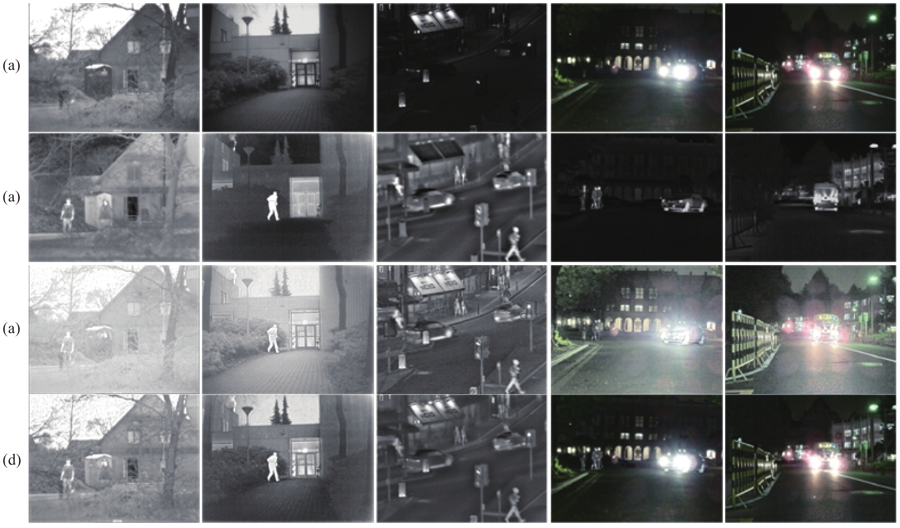
所提出模型具备环境感知能力,在不同的场景下呈现出不同的功能,这是由于使用了基于CLIP的场景信息感知模块. CLIP不仅具备图像编码器,其同样具备文本编码器,一些明暗并不明显的场景,使用CLIP模型可能无法做出正确的场景理解,当算法应用到真实场景中会存在巨大的隐患. 为了保证所提出模型在一些无法判断的场景下依旧可以正确使用,提升模型的实用性,本文尝试构建了文本引导的多场景图像融合算法. 文本引导和图像引导具备完全相同的架构,只是文本引导模型的场景信息感知模块的输入由图像切换为文本. 图11中呈现了使用不同引导语句,融合网络所呈现出的不同融合结果. 融合图像1的引导语句为“黑暗场景下的融合任务”,融合图像2的引导语句为“正常亮度场景下的图像融合任务
![]() 图 11 不同引导语句下的融合结果. (a)可见光图像;(b)红外图像;(c)融合图像1;(d)融合图像2Figure 11. Fusion results under different boot statements: (a) the visible image, (b) the infrared image, (c) the fusion Image 1, and (d) the fusion Image 2
图 11 不同引导语句下的融合结果. (a)可见光图像;(b)红外图像;(c)融合图像1;(d)融合图像2Figure 11. Fusion results under different boot statements: (a) the visible image, (b) the infrared image, (c) the fusion Image 1, and (d) the fusion Image 22.11 效率分析
表9中呈现了所提算法在Nvidia
3090 上的运行效率分析. 由于本文模型借助大模型实现不同环境下的图像融合任务,因此在模型大小和计算量的统计上,受到大模型的影响,并没有处于一个很低的水平. 但是大模型只负责在测试阶段对输入的场景进行理解和编码,因此所提出方法具备适中的计算量和测试时间,可以在0.35 s内处理一对可见光和红外图像. 当环境变得更加复杂,模型可以以适中的计算代价实现微调,以适应更加极端的环境. 在未来的工作中,本文将持续对模型的结构进行优化,以进一步提升模型的轻量性,保证其可以被部署到合适的终端设备上.表 9 在Nvidia3090上的模型效率分析Table 9. Analysing the efficiency of the model on the Nvidia3090Method Model Size Flops/GB Test time/s DenseFuse[9] 1.02 59.24 0.05 FusionGAN[13] 7.24 39.91 0.08 GANMcC[12] 1.09 93.36 0.05 RFN-Nest[10] 28.70 102.64 0.06 SuperFusion[23] 22.40 76.67 0.04 SwinFusion[17] 52.71 398.32 0.73 UMF-CMGR[24] 7.22 193.24 0.01 LRRNet[25] 0.21 40.05 0.07 DATFuse[26] 0.07 21.66 0.02 MLFFusion[27] 4.52 53.21 0.04 ResCCFusion[28] 0.87 102.62 0.06 Ours 104.58 185.2 0.35 3. 结论
本文针对现有的图像融合方法在复杂光照环境下成像不稳定的问题,提出了一个具备场景理解功能的多场景图像融合网络. 通过设计基于状态空间方程的特征提取模块、粒度渐进的融合规则和基于大模型的场景信息嵌入模块,实现了在不同极端光照环境下表现较好的图像融合算法. 主要得出以下结论:
(1)本文设计了基于状态空间方程的特征提取模块,以线性的复杂度实现了全局的信息感知能力,有效地提升了模型的特征表达能力,实现了对图像的全局结构化建模.
(2)针对现有多模态融合模型的不足,本文提出了一种粒度渐进的融合规则,通过结合序列化模型和卷积模型的优点,从全局到局部渐进地整合差异巨大的多模态特征,有效地解决了多模态特征融合不充分的问题.
(3)提出了基于大模型的场景信息嵌入模块,通过预训练的CLIP图像编码器对可见光图像进行编码,接着使用KAN层处理编码向量,并利用编码向量逐层、逐通道地调控融合特征,使图像融合模型可以根据场景的变换生成风格不同的融合图像,保证了融合模型可以在各种极端光照环境下都可以获得极佳的视觉效果.
(4)在暗光数据集LLVIP和MSRS,道路场景数据集RoadScene,军事场景数据集TNO和包含雾霾场景的数据集M3FD上,本文模型与11种最先进的方法相比均取得了更好的定性和定量效果.
所提出算法在自动驾驶、故障诊断、战场侦察等领域表现出较大的应用前景. 在未来的工作中,将继续整合更多复杂场景,以构建通用的、全天候的图像融合网络,进一步拓展所提出方法的应用场景.
-
![]()
图 1 整体的网络结构图. (a)整体网络结构; (b)粒度渐进融合模块; (c)场景信息融合模块; (d)特征空间的变化
Figure 1. Overall network structure diagram: (a) overall network; (b) Progressive Granular Fusion Module; (c) Scene Information Embedding Module; (d) variation of the feature space
![]()
图 2 在MSRS数据集上进行定性对比的结果. (a)可见光图像; (b)红外图像; (c) DATFuse生成的图像; (d) DenseFuse生成的图像; (e) FusionGAN生成的图像; (f) GANMcC生成的图像; (g) LRRNet生成的图像; (h) MLFFusion生成的图像; (i) ResCCFusion生成的图像; (j) RFN-Nest生成的图像; (k) SuperFusion生成的图像; (l) SwinFusion生成的图像; (m) UMF-CMGR生成的图像; (n)本文方法生成的图像
Figure 2. Results of the qualitative comparison on the MSRS dataset: (a) the visible image; (b) the infrared image; (c) the image generated by DATFuse; (d) the image generated by DenseFuse; (e) the image generated by FusionGAN; (f) the image generated by GANMcC; (g) the image generated by LRRNet; (h) the image generated by MLFFusion; (i) the image generated by ResCCFusion; (j) the image generated by RFN-Nest; (k) the image generated by SuperFusion; (l) the image generated by SwinFusion; (m) the image generated by UMF-CMGR; (n) the image generated by the proposed method
![]()
图 3 在TNO数据集上进行定性对比的结果. (a)可见光图像; (b)红外图像; (c) DATFuse生成的图像; (d) DenseFuse生成的图像; (e) FusionGAN生成的图像; (f) GANMcC生成的图像; (g) LRRNet生成的图像; (h) MLFFusion生成的图像; (i) ResCCFusion生成的图像; (j) RFN-Nest生成的图像; (k) SuperFusion生成的图像; (l) SwinFusion生成的图像; (m) UMF-CMGR生成的图像; (n)本文方法生成的图像
Figure 3. Results of the qualitative comparison on the TNO dataset: (a) the visible image; (b) the infrared image; (c) the image generated by DATFuse; (d) the image generated by DenseFuse; (e) the image generated by FusionGAN; (f) the image generated by GANMcC; (g) the image generated by LRRNet; (h) the image generated by MLFFusion; (i) the image generated by ResCCFusion; (j) the image generated by RFN-Nest; (k) the image generated by SuperFusion; (l) the image generated by SwinFusion; (m) the image generated by UMF-CMGR; (n) the image generated by the proposed method
![]()
图 4 在LLVIP数据集上进行定性对比的结果. (a)可见光图像; (b)红外图像; (c) DATFuse生成的图像; (d) DenseFuse生成的图像; (e) FusionGAN生成的图像; (f) GANMcC生成的图像; (g) LRRNet生成的图像; (h) MLFFusion生成的图像; (i) ResCCFusion生成的图像; (j) RFN-Nest生成的图像; (k) SuperFusion生成的图像; (l) SwinFusion生成的图像; (m) UMF-CMGR生成的图像; (n)本文方法生成的图像
Figure 4. Results of the qualitative comparisons on the LLVIP dataset: (a) the visible image; (b) the infrared image; (c) the image generated by DATFuse; (d) the image generated by DenseFuse; (e) the image generated by FusionGAN; (f) the image generated by GANMcC; (g) the image generated by LRRNet; (h) the image generated by MLFFusion; (i) the image generated by ResCCFusion; (j) the image generated by RFN-Nest; (k) the image generated by SuperFusion; (l) the image generated by SwinFusion; (m) the image generated by UMF-CMGR; (n) the image generated by the proposed method
![]()
图 5 在M3FD数据集上进行定性对比的结果. (a)可见光图像; (b)红外图像; (c) DATFuse生成的图像; (d) DenseFuse生成的图像; (e) FusionGAN生成的图像; (f) GANMcC生成的图像; (g) LRRNet生成的图像; (h) MLFFusion生成的图像; (i) ResCCFusion生成的图像; (j) RFN-Nest生成的图像; (k) SuperFusion生成的图像; (l) SwinFusion生成的图像; (m) UMF-CMGR生成的图像; (n)本文方法生成的图像
Figure 5. Results of the qualitative comparisons on the M3FD dataset: (a) the visible image; (b) the infrared image; (c) the image generated by DATFuse; (d) the image generated by DenseFuse; (e) the image generated by FusionGAN; (f) the image generated by GANMcC; (g) the image generated by LRRNet; (h) the image generated by MLFFusion; (i) the image generated by ResCCFusion; (j) the image generated by RFN-Nest; (k) the image generated by SuperFusion; (l) the image generated by SwinFusion; (m) the image generated by UMF-CMGR; (n) the image generated by the proposed method
![]()
图 6 在RoadScene数据集上选取日间环境进行定性对比的结果. (a)可见光图像; (b)红外图像; (c) DATFuse生成的图像; (d) DenseFuse生成的图像; (e) FusionGAN生成的图像; (f) GANMcC生成的图像; (g) LRRNet生成的图像; (h) MLFFusion生成的图像; (i) ResCCFusion生成的图像; (j) RFN-Nest生成的图像; (k) SuperFusion生成的图像; (l) SwinFusion生成的图像; (m) UMF-CMGR生成的图像; (n)本文方法生成的图像
Figure 6. Results of the qualitative comparisons on the RoadScene dataset in daytime: (a) the visible image; (b) the infrared image; (c) the image generated by DATFuse; (d) the image generated by DenseFuse; (e) the image generated by FusionGAN; (f) the image generated by GANMcC; (g) the image generated by LRRNet; (h) the image generated by MLFFusion; (i) the image generated by ResCCFusion; (j) the image generated by RFN-Nest; (k) the image generated by SuperFusion; (l) the image generated by SwinFusion; (m) the image generated by UMF-CMGR; (n) the image generated by the proposed method
![]()
图 7 在RoadScene数据集上选取夜间环境进行定性对比的结果(a)可见光图像; (b)红外图像; (c) DATFuse生成的图像; (d) DenseFuse生成的图像; (e) FusionGAN生成的图像; (f) GANMcC生成的图像; (g) LRRNet生成的图像; (h) MLFFusion生成的图像; (i) ResCCFusion生成的图像; (j) RFN-Nest生成的图像; (k) SuperFusion生成的图像; (l) SwinFusion生成的图像; (m) UMF-CMGR生成的图像; (n)本文方法生成的图像
Figure 7. Results of the qualitative comparisons on theRoadScene dataset in nighttime: (a) the visible image; (b) the infrared image; (c) the image generated by DATFuse; (d) the image generated by DenseFuse; (e) the image generated by FusionGAN; (f) the image generated by GANMcC; (g) the image generated by LRRNet; (h) the image generated by MLFFusion; (i) the image generated by ResCCFusion; (j) the image generated by RFN-Nest; (k) the image generated by SuperFusion; (l) the image generated by SwinFusion; (m) the image generated by UMF-CMGR; (n) the image generated by the proposed method
![]()
图 8 在MSRS数据集上级联方法进行定性对比的结果 (a)可见光图像; (b)红外图像; (c) DATFuse生成的图像; (d) DenseFuse生成的图像; (e) FusionGAN生成的图像; (f) GANMcC生成的图像; (g) LRRNet生成的图像; (h) MLFFusion生成的图像; (i) ResCCFusion生成的图像; (j) RFN-Nest生成的图像; (k) SuperFusion生成的图像; (l) SwinFusion生成的图像; (m) UMF-CMGR生成的图像; (n)本文方法生成的图像
Figure 8. Results of the qualitative comparisons of cascade methods on the MSRS dataset: (a) the visible image; (b) the infrared image; (c) the image generated by DATFuse; (d) the image generated by DenseFuse; (e) the image generated by FusionGAN; (f) the image generated by GANMcC; (g) the image generated by LRRNet; (h) the image generated by MLFFusion; (i) the image generated by ResCCFusion; (j) the image generated by RFN-Nest; (k) the image generated by SuperFusion; (l) the image generated by SwinFusion; (m) the image generated by UMF-CMGR; (n) the image generated by the proposed method
![]()
图 9 模块消融实验对比效果图. (a)可见光图像;(b)红外图像;(c)移除粒度渐进融合模块后生成的融合图像;(d)移除场景信息感知模块后生成的融合图像;(e)本文方法生成的融合图像.
Figure 9. Visual contrast rendering of the module ablation experiment: (a)the visible light image; (b) the infrared image; (c) the fused image generated after removing the granularity-progressive fusion module; (d) the fused image generated after removing the scene information perception module; (e) the fused image generated by the proposed method.
![]()
图 10 特征提取模块消融实验的视觉对比效果图. (a)可见光图像;(b)红外图像;(c)基于CNN框架的网络生成的图像;(d)基于Transformer框架的网络生成的图像;(e)本文框架生成的融合图像.
Figure 10. Visual comparison of the effect of the feature extraction module ablation experiment: (a) the visible image; (b) the infrared image; (c) the fused image generated by the CNN framework; (d) the fused image generated by the Transformer framework; (e) the fused image generated by the proposed method.
![]()
图 11 不同引导语句下的融合结果. (a)可见光图像;(b)红外图像;(c)融合图像1;(d)融合图像2
Figure 11. Fusion results under different boot statements: (a) the visible image, (b) the infrared image, (c) the fusion Image 1, and (d) the fusion Image 2
表 1 在MSRS数据集上的定量对比
Table 1 Quantitative comparison on the MSRS datasets
Method Year SD VIF AG EN Qabf SF DenseFuse[9] 2019 21.7389 0.7632 1.8535 5.5269 0.4382 5.6679 FusionGAN[13] 2019 17.1449 0.4132 1.2088 5.2505 0.1382 3.8752 GANMcC[12] 2021 24.3486 0.6825 1.8351 5.8325 0.3384 5.2267 RFN-Nest[10] 2021 21.5879 0.5741 1.2661 5.3887 0.2417 4.3374 SuperFusion[23] 2022 32.1587 0.9169 2.5704 5.9026 0.5886 8.5035 SwinFusion[17] 2022 32.8862 0.9570 2.6751 5.9138 0.5806 8.7782 UMF-CMGR[24] 2022 16.8892 0.3084 1.7376 5.0580 0.2320 6.0331 LRRNet[25] 2023 20.3234 0.4362 1.6918 5.1835 0.3084 6.0885 DATFuse[26] 2023 27.0892 0.8493 2.6178 5.8089 0.5418 8.8730 ResCCFusion[27] 2024 29.8823 0.9416 2.5002 5.8360 0.6294 8.3571 MLFFusion[28] 2023 33.3281 0.9769 3.0618 5.8053 0.6311 9.6072 Ours 47.8841 1.2566 6.0620 7.2697 0.3043 15.6929  下载: 导出CSV
表 2 在TNO数据集上的定量对比
Table 2 Quantitative comparison on the TNO datasets
Method SD VIF AG EN Qabf SF DenseFuse[9] 34.8425 0.6630 3.5432 6.8206 0.4471 8.9475 FusionGAN[13] 30.7810 0.4244 2.4184 6.5572 0.2343 6.2719 GANMcC[12] 33.4233 0.5324 2.5204 6.7338 0.2787 6.1114 RFN-Nest[10] 36.9403 0.5614 2.6541 6.9661 0.3334 5.8461 SuperFusion[23] 37.0824 0.6858 3.5658 6.7629 0.4757 9.2355 SwinFusion[17] 39.7786 0.7651 4.2170 6.9082 0.5261 10.7610 UMF-CMGR[24] 30.1167 0.5981 2.9691 6.5371 0.4114 8.1779 LRRNet[25] 40.9867 0.5636 3.7621 6.9909 0.3533 9.5100 DATFuse[26] 28.3505 0.7301 3.6975 6.5507 0.5227 10.0466 ResCCFusion[27] 40.7118 0.8277 3.8048 7.0003 0.5195 10.0035 MLFFusion[28] 41.4123 0.7548 4.0195 6.9071 0.5192 10.0094 Ours 39.5807 0.6670 4.5763 6.9438 0.5265 11.9243
下载: 导出CSV
表 3 在LLVIP数据集上的定量对比
Table 3 Quantitative comparison on the LLVIP datasets
Method SD VIF AG EN Qabf SF DenseFuse[9] 34.1926 0.7669 2.7220 6.8751 0.4885 9.2664 FusionGAN[13] 24.8206 0.4762 1.9468 6.3083 0.2539 6.9194 GANMcC[12] 32.1132 0.6125 2.1229 6.6899 0.2972 6.8144 RFN-Nest[10] 34.6463 0.6693 2.1579 6.8624 0.3129 6.3211 SuperFusion[23] 42.3495 0.8180 3.1196 7.1280 0.5281 11.1390 SwinFusion[17] 44.9182 0.9324 3.9154 7.1586 0.6489 13.6233 UMF-CMGR[24] 29.3794 0.5208 2.5041 6.4620 0.3473 9.9154 LRRNet[25] 24.8671 0.5640 2.4671 6.1452 0.4242 9.1082 DATFuse[26] 39.8505 0.8388 3.0364 7.0820 0.5136 12.3311 ResCCFusion[27] 24.8671 0.5640 2.4671 6.1452 0.4242 9.1082 MLFFusion[28] 46.5614 0.9596 4.0846 7.2267 0.6751 13.9526 Ours 43.5546 1.0832 7.5902 7.3343 0.3263 23.1897
下载: 导出CSV
表 4 在M3FD定量对比
Table 4 Quantitative comparison on the M3FD datasets
Method SD VIF AG EN Qabf SF DenseFuse[9] 26.1373 0.7985 2.3549 6.6033 0.5199 7.1329 FusionGAN[13] 27.8432 0.5656 2.3499 6.7448 0.3377 6.6424 GANMcC[12] 30.4889 0.5040 1.9505 6.8846 0.2841 5.5501 RFN-Nest[10] 32.1853 0.6962 2.0794 6.9956 0.4214 5.7635 SuperFusion[23] 17.7198 0.8197 2.2826 5.9919 0.5455 7.1204 SwinFusion[17] 19.0168 0.8721 2.5661 6.0927 0.5638 7.8699 UMF-CMGR[24] 24.0267 0.6658 1.7974 6.5609 0.3735 5.6679 LRRNet[25] 19.4493 0.6445 2.6237 6.2279 0.4695 8.3066 DATFuse[26] 13.4647 0.6995 2.5456 5.6910 0.5116 7.9709 ResCCFusion[27] 25.0947 0.6918 2.9221 6.6176 0.4440 9.0550 MLFFusion[28] 17.4232 0.9546 2.5260 5.9499 0.6028 7.9004 Ours 47.0762 0.7902 5.2970 7.0008 0.3046 16.5346
下载: 导出CSV
表 5 在RoadScene定量对比
Table 5 Quantitative comparison on the RoadScene datasets
Method SD VIF AG EN Qabf SF DenseFuse[9] 41.6418 0.5663 5.1588 7.2664 0.4679 13.3948 FusionGAN[13] 38.6246 0.3528 3.5230 7.0938 0.2573 9.0313 GANMcC[12] 44.3764 0.4776 4.0184 7.3113 0.3286 9.4598 RFN-Nest[10] 45.6429 0.4871 3.7070 7.3672 0.3104 8.6350 SuperFusion[23] 42.2997 0.5884 4.7654 7.0008 0.4459 13.0590 SwinFusion[17] 44.5553 0.5879 4.8509 7.0231 0.4379 12.9205 UMF-CMGR[24] 35.2428 0.5478 4.6126 7.0400 0.4427 12.0836 LRRNet[25] 43.3252 0.4882 5.0379 7.1686 0.3602 13.3470 DATFuse[26] 29.9707 0.5481 4.3028 6.7718 0.4439 12.0730 ResCCFusion[27] 50.5523 0.6253 5.3980 7.4612 0.4914 14.2099 MLFFusion[28] 41.9363 0.6863 4.5580 7.0460 0.4614 13.0562 Ours 46.7927 0.7513 6.5371 7.3818 0.6184 17.2539
下载: 导出CSV
表 6 在MSRS数据集上级联方法的定量指标对比
Table 6 Comparison of quantitative metrics for cascade methods on the MSRS dataset
Method SD VIF AG EN Qabf SF DenseFuse[9] 36.3769 1.0095 3.5126 5.9035 0.5453 9.6305 FusionGAN[13] 26.7274 0.5313 2.1367 6.1548 0.2406 6.2425 GANMcC[12] 39.6900 0.8603 3.3213 6.7057 0.4334 8.4948 RFN-Nest[10] 36.1940 0.7463 2.2290 6.3065 0.3672 6.8413 SuperFusion[23] 45.4127 1.0689 4.3345 6.7453 0.4551 11.9034 SwinFusion[17] 46.5278 1.0874 4.4845 6.7618 0.4247 12.3741 UMF-CMGR[24] 25.1042 0.3768 3.1528 6.0111 0.3112 9.1723 LRRNet[25] 31.5402 0.5071 3.0804 5.5901 0.3694 9.8270 DATFuse[26] 39.3817 1.0232 4.4120 6.2832 0.3636 13.0349 MLFFusion[27] 45.7913 1.0994 5.2045 6.6393 0.3541 13.8107 ResCCFusion[28] 43.7759 1.2038 4.3400 6.2440 0.4877 12.3908 Ours 47.8841 1.2566 6.0620 7.2697 0.3043 15.6929
下载: 导出CSV
表 7 模块消融实验的定量对比
Table 7 Quantitative comparison of module ablation experiments.
Method SD VIF AG EN Qabf SF A 46.3691 1.2097 5.0382 7.1851 0.2812 13.716 B 34.8423 0.9917 3.5474 6.4095 0.5463 10.105 Ours 47.8841 1.2566 6.0620 7.2697 0.3043 15.6929 Notes:A represents the network with the granularity-progressive fusion module removed, and B represents the network with the scene information perception module removed
下载: 导出CSV
表 8 特征提取模块消融实验的定量对比
Table 8 Quantitative comparison of feature extraction module ablation experiments
Feature Extraction SD VIF AG EN Qabf SF CNN based method 45.1432 1.2545 5.0845 7.2445 0.2967 13.781 Transformer based method 46.7344 1.0864 5.4136 7.1731 0.3065 14.441 Ours 47.8841 1.2566 6.0620 7.2697 0.3043 15.6929
下载: 导出CSV
表 9 在Nvidia3090上的模型效率分析
Table 9 Analysing the efficiency of the model on the Nvidia3090
Method Model Size Flops/GB Test time/s DenseFuse[9] 1.02 59.24 0.05 FusionGAN[13] 7.24 39.91 0.08 GANMcC[12] 1.09 93.36 0.05 RFN-Nest[10] 28.70 102.64 0.06 SuperFusion[23] 22.40 76.67 0.04 SwinFusion[17] 52.71 398.32 0.73 UMF-CMGR[24] 7.22 193.24 0.01 LRRNet[25] 0.21 40.05 0.07 DATFuse[26] 0.07 21.66 0.02 MLFFusion[27] 4.52 53.21 0.04 ResCCFusion[28] 0.87 102.62 0.06 Ours 104.58 185.2 0.35
下载: 导出CSV
-
[1] Yao J X, Zhao Y Q, Bu Y Y, et al. Laplacian pyramid fusion network with hierarchical guidance for infrared and visible image fusion. IEEE Trans Circuits Syst Video Technol, 2023, 33(9): 4630 doi: 10.1109/TCSVT.2023.3245607
[2] 马忠贵, 李卓, 梁彦鹏. 自动驾驶车联网中通感算融合研究综述与展望. 工程科学学报, 2023, 45(1):137 Ma Z G, Li Z, Liang Y P. Overview and prospect of communication-sensing-computing integration for autonomous driving in the internet of vehicles. Chin J Eng, 2023, 45(1): 137
[3] Yang Y, Liu J X, Huang S Y, et al. Infrared and visible image fusion via texture conditional generative adversarial Network. IEEE Trans Circuits Syst Video Technol, 2021, 31(12): 4771 doi: 10.1109/TCSVT.2021.3054584
[4] 王瑞琳, 王立, 贺盈波. 基于小波和动态互补滤波的图像与事件融合方法. 工程科学学报, 2024, 46(11):2076 Wang R L, Wang L, He Y B. Image and event fusion method based on wavelet and dynamic complementary filtering. Chin J Eng, 2024, 46(11): 2076
[5] Tang L F, Zhang H, Xu H, et al. Rethinking the necessity of image fusion in high-level vision tasks: A practical infrared and visible image fusion network based on progressive semantic injection and scene fidelity. Inf Fusion, 2023, 99: 101870 doi: 10.1016/j.inffus.2023.101870
[6] Wang Z S, Shao W Y, Chen Y L, et al. A cross-scale iterative attentional adversarial fusion network for infrared and visible images. IEEE Trans Circuits Syst Video Technol, 2023, 33(8): 3677 doi: 10.1109/TCSVT.2023.3239627
[7] Li X L, Li Y F, Chen H J, et al. CCAFusion: Cross-modal coordinate attention network for infrared and visible image fusion. IEEE Trans Circuits Systr Video Technol, 2024, 34(2): 866 doi: 10.1109/TCSVT.2023.3293228
[8] Park S, Vien A G, Lee C, et al. Cross-modal transformers for infrared and visible image fusion. IEEE Trans Circuits Syst Video Technol, 2024, 34(2): 770 doi: 10.1109/TCSVT.2023.3289170
[9] Gao Y , Ma S W, Liu J J, et al. DCDR-GAN: A densely connected disentangled representation generative adversarial network for infrared and visible image fusion. IEEE Trans Circuits Syst Video Technol, 2023, 33(2): 549
[10] Li H, Wu X J, Kittler J. RFN-Nest: An end-to-end residual fusion network for infrared and visible images. Inf Fusion, 2021, 73: 72 doi: 10.1016/j.inffus.2021.02.023
[11] Li H, Wu X J. DenseFuse: A fusion approach to infrared and visible images. IEEE Trans Image Process, 2019, 28(5): 2614 doi: 10.1109/TIP.2018.2887342
[12] Ma J Y, Zhang H, Shao Z F et al. GANMcC: A generative adversarial network with multiclassification constraints for infrared and visible image fusion. IEEE Trans Instrum Meas, 2021, 70: 5005014
[13] Ma J Y, Yu W, Liang P W, et al. FusionGAN: A generative adversarial network for infrared and visible image fusion. Inf Fusion, 2019, 48: 11 doi: 10.1016/j.inffus.2018.09.004
[14] Yue J, Fang L Y, Xia S B et al. Dif-fusion: Toward high color fidelity in infrared and visible image fusion with diffusion models. IEEE Trans Image Process, 2023, 32: 5705 doi: 10.1109/TIP.2023.3322046
[15] Li H, Wu X J, CrossFuse: A novel cross attention mechanism based infrared and visible image fusion approach. Inf Fusion, 2024, 103: 102147
[16] Ma L, Ma T Y, Liu R S, et al. Toward fast, flexible, and robust low-light image enhancement // 2023 IEEE/CVF Conference on Computer Vision and Pattern Recognition. Vancouver, 2023: 5637
[17] Ma J Y, Tang L F, Fan F et al. SwinFusion: Cross-domain long-range learning for general image fusion via swin transformer. IEEE/CAA J Autom Sin, 2022, 9(7): 1200 doi: 10.1109/JAS.2022.105686
[18] Tang L F , Yuan J T , Zhang H, et al. PIAFusion: A progressive infrared and visible image fusion network based on illumination aware. Inf Fusion, 2022, 83: 79
[19] Tang L F, Xiang X Y, Zhang H, et al. DIVFusion: Darkness-free infrared and visible image fusion. Inf Fusion, 2023, 91: 477 doi: 10.1016/j.inffus.2022.10.034
[20] 唐霖峰, 张浩, 徐涵. 基于深度学习的图像融合方法综述. 中国图象图形学报, 2023, 28(1):3 Tang L F, Zhang H, Xu H. Deep learning-based image fusion: a survey. J Image Graph. 2023, 28(1): 3
[21] 孙彬, 高云翔, 诸葛吴为. 可见光与红外图像融合质量评价指标分析. 中国图象图形学报, 2023, 28(1):144 Sun B, Gao Y X, Zhuge W W. Analysis of quality objective assessment metrics for visible and infrared image fusion. J Image Graph. 2023, 28(1): 144
[22] Tan M J, Gao S B, Xu W Z, et al. Visible-infrared image fusion based on early visual information processing mechanisms. IEEE Trans Circuits Syst Video Technol, 2021, 31(11): 4357 doi: 10.1109/TCSVT.2020.3047935
[23] Tang L F, Deng Y X, Ma Y, et al. SuperFusion: A versatile image registration and fusion network with semantic awareness. IEEE/CAA J Autom Sin, 2022, 9(12): 2121 doi: 10.1109/JAS.2022.106082
[24] Wang D, Liu J Y, Fan X, et al. Unsupervised Misaligned Infrared and Visible Image Fusion via Cross-Modality Image Generation and Registration // International Joint Conference on Artificial Intelligence. Vienna, 2022: 3256
[25] Li H, Xu T Y, Wu X J, et al. LRRNet: A novel representation learning guided fusion network for infrared and visible images. IEEE Trans Pattern Anal Mach Intell, 2023, 45(9): 11040 doi: 10.1109/TPAMI.2023.3268209
[26] Tang W, He F Z, Liu Y, et al. DATFuse: Infrared and visible image fusion via dual attention transformer. IEEE Trans Circuits Systr Video Technol, 2023, 33(7): 3159 doi: 10.1109/TCSVT.2023.3234340
[27] Wang C Y, Sun D D, Gao Q, et al. MLFFusion: Multi-level feature fusion network with region illumination retention for infrared and visible image fusion. Infrared Phys Technol, 2023, 134: 104916 doi: 10.1016/j.infrared.2023.104916
[28] Xiong Z, Zhang X H, Han H W, et al. ResCCFusion: Infrared and visible image fusion network based on ResCC module and spatial criss-cross attention models. Infrared Phys Technol, 2024, 136: 104962 doi: 10.1016/j.infrared.2023.104962
计量
- 文章访问数: 391
- HTML全文浏览量: 91
- PDF下载量: 42
